GA-CCRi Analytical Development Services

Representing entities by their attributes, like just about any database does, makes it easy to manipulate information about these entities using their attribute values—for example, to list all the employees who have “Shipping” as their “Department” value. The popular machine learning approach of representing entities as vectors created by neural networks lets us identify similarities and relationships (embedded in a “vector space”) that might not be apparent with a more traditional approach, although the black box nature of some of these systems frustrates many users who want to understand more about the nature of the relationships. Our experiments demonstrate methods for combining these techniques that let us use attribute values to tune the use of vector embeddings and get the best of both worlds.

In order to implement this, your data must be represented as tensors, which are a generalization of scalars, vectors, and matrices, to potentially higher dimensions. For many applications, this is already the case. If you are looking at the history of a stock’s price, that data can be represented as a 1-tensor (vector) of floating point values. If you are trying to analyze a photograph, it can be represented as a 3-tensor containing the red, green, and blue values of each pixel. For other applications, such as dealing with text or entities (persons, places, organizations), this gets a little trickier.

The simplest way to represent such data as a tensor is using a one-hot (dummy) encoding.

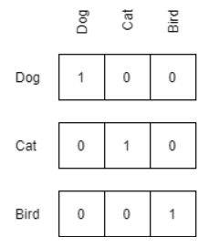
This has the advantage of uniquely encoding each entity in your data, but it has the disadvantage of being memory-intensive for large datasets. (The memory footprint can be reduced if your tensor library supports sparse tensors, but this typically limits the variety of operations that can be performed.) This approach also suggests that all entities are orthogonal—in other words, it assumes that the words puppy and dog are just as dissimilar as potato and dog.

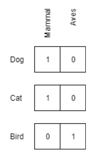
Entities can also be represented in terms of their attributes or properties, if such data is available. Such encodings have the advantage of being entirely transparent, which is useful when using them as features for other models. This lets us manually scale and weight different features to emphasize or de-emphasize their impact on the model.

You can also use an unsupervised embedding approach to represent the data. Techniques such as GloVe, word2vec, and fastText distribute each entity as points in a continuous vector space such that similar words inhabit locations near to one another. In the following, columns represent coordinates in this vector space:

What if we want to combine the use of attributes with the use of vector space embeddings? The obvious solution is to simply concatenate the vectors, but this has some complications due to information being duplicated. Information that is explicitly encoded in the attribute vectors is also implicitly encoded in the embeddings, which takes away our ability to vary the emphasis on certain features if we want to tune the model’s usage of different attributes. Essentially, what we want is an attribute vector that explicitly represents the known properties of an entity and an embedding vector containing any latent information that is “left over”.

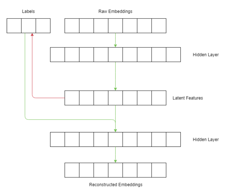
To accomplish this, we combine the principles from two different types of neural network architectures: generative adversarial networks (GANs) and autoencoders. As Wikipedia describes it, an autoencoder is a type of artificial neural network used to learn efficient data codings in an unsupervised manner. An autoencoder aims to learn a representation (encoding) for a set of data, typically for the purpose of dimensionality reduction. It learns to encode and transform the inputs so that the maximum amount of information is retained by ensuring that the encodings can be used to reconstruct the original input. In our experiments, we also use a simple linear mapping that attempts to reconstruct the attribute vector from the latent encodings. This reconstruction loss is also considered by the autoencoder, which it tries to minimize, making these two networks “adversarial”.

Specifically, the autoencoder is comprised of an encoder network ϕ and a decoder network ψ, with one key difference: the attribute vector is concatenated to the encodings before being passed through the the decoder network. Since the objective is to remove attribute information from the encodings, we cannot expect the decoder to reconstruct the original input with just the encodings. By including the raw attribute values to the input of the decoder, we are giving it access to all of the information necessary to reconstruct the original input.

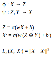
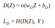
During training, the autoencoder tries to simultaneously minimize is reconstruction loss while maximizing the discriminator’s cross-entropy loss.

In short, we are trying to learn a new representation of the embeddings that cannot be mapped back to the attributes, but when combined with the attributes can be mapped back to the original embeddings.

To test how well this network works, we use fastText word vectors trained on the Wikipedia corpus as our entity embeddings and WordNet properties as our attributes. Specifically, we consider all of the words in WordNet with the property “animal”. As a very simple test, we try to isolate information about the label “canine” from the fastText embeddings. The embedding space diagram below shows them as yellow circles outlined in black.

As we would expect, initially words with the label “canine” end up mostly concentrated in small clusters in the embedding space:

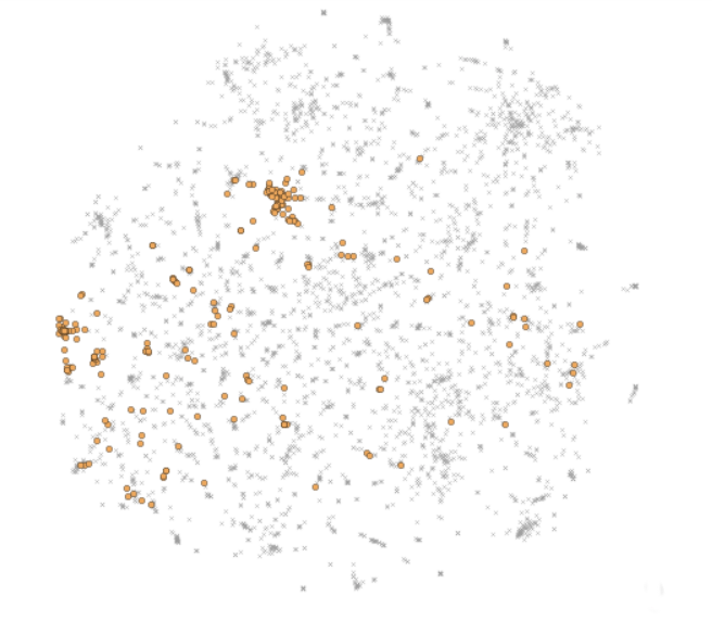
However, after training the network and passing the embeddings though it to be encoded, words with the label “canine” end up being fairly uniformly distributed in the space:

We can further interpret the effect of this transformation by looking at nearest neighbors in the embedding space. The most similar words to “dog” in the original fastText embeddings are all types of dog:

1. Puppy
2. Dachshund
3. Poodle
4. Coonhound
5. Doberman
6. Hound
7. Terrier
8. Retriever

In the transformed embeddings, with canine information removed, the nearest neighbors are a mix of types of housepets and dogs:

1. Cat
2. Hamster
3. Doberman
4. Kitten
5. Puppy
6. Rabbit
7. Mouse
8. Dachshund

We also want to ensure that the inclusion and exclusion of canine-ness has little to no effect on the nearest neighbors of non-canine entities. In the original space, the nearest neighbors to “crab” are as follows:

1. Lobster
2. Shrimp
3. Crayfish
4. Clam
5. Crustacean
6. Prawn
7. Mackerel
8. Octopus

And in the transformed space:

1. Lobster
2. Clam
3. Shrimp
4. Octopus
5. Prawn
6. Geoduck
7. Oyster
8. Squid

Ideally, these lists would be identical, so the result isn’t perfect, but they are quite similar.

Alternatively, instead of ignoring canine-ness we can emphasize that aspect of our representations. In the original fastText embeddings, the nearest neighbors to “wolf” are the following:

1. Grizzly
2. Coyote
3. Raccoon
4. Jackal
5. Dog
6. Bear
7. Bison
8. Boar

This result is understandable. Aside from the generic “dog” these are mostly wild animals that inhabit similar biomes. What if we want to emphasize the fact that wolves are canines? We can increase the weight of that dimension of our hybrid embedding, which results in the following:

1. Coyote
2. Jackal
3. Redbone
4. Dog
5. Fox
6. Raccoon
7. Bluetick
8. Doberman

Now, wild dogs such as coyote, jackal, and fox are all considered more similar to wolf, while racoon falls from 3rd to 6th, and grizzly, bear, bison, and boar and fall off completely. The tuning of that dimension has improved the nearest-neighbors calculations.

Next, we would repeat the training mentioned earlier but with more attributes being isolated: canine, feline, mammal. We can now have some fun with finding the nearest neighbors to words while altering their attributes. For example, what are the nearest neighbors to “dog” if instead of being canine it was feline?

1. Feline
2. Tabby
3. Angora
4. Tigress
5. Kitty
6. Bobcat
7. Lioness
8. Cougar

The five most similar entities to a dog, if it were feline instead of canine, are types of housecat! Similarly, we can look at the most similar entities to “dog” if it were not a mammal:

1. Pet
2. Animal
3. Chicken
4. Goose
5. Mouthbreeder
6. Tortoise
7. Newt
8. Goldfish

Which results in non-mammalian animals that are either common farm animals or pets.

Conclusion

We introduce a method for combining unsupervised representations of data with attribute labels into a unified hybrid representation. A novel neural network architecture containing an autoencoder and GAN effectively isolates these attribute labels from the rest of the latent embedding. Using fastText word vectors as embeddings and WordNet hyponym relations from WordNet, we demonstrated the viability of this approach. Finally, we saw the power of the resulting hybrid embeddings for semantic search, where certain aspects of a query can be (de)emphasized and hypothetical “what if” queries can be made where properties can be toggled on and off.

Over the past few years, the use of embeddings to identify entity similarity has been a great benefit to all kinds of search applications, because the use of semantics can do much more than simple string searches or the use of labor-intensive taxonomies. The incorporation of attribute labels into this system—especially when this includes the ability to manually tune their effect—brings even greater power to this approach.