GA-CCRi Analytical Development Services

At GA-CCRi our primary goal is to extract useful information from the data we process. We’re constantly striving to improve our data processing tools to enable powerful workflows and easier development. In October 2022 we released updates to our open source project GeoMesa that enables integrations with Kafka Streams. This allows us to leverage the stream processing capabilities of Kafka Streams on our existing GeoMesa Kafka topics, to easily produce spatial streaming analytics. 

Streaming Spatial Data in Kafka

For many years GeoMesa has integrated with Kafka to provide streaming spatial data. This technology is used to power our live views and render live layers in GeoServer or other GeoTools datastore applications.

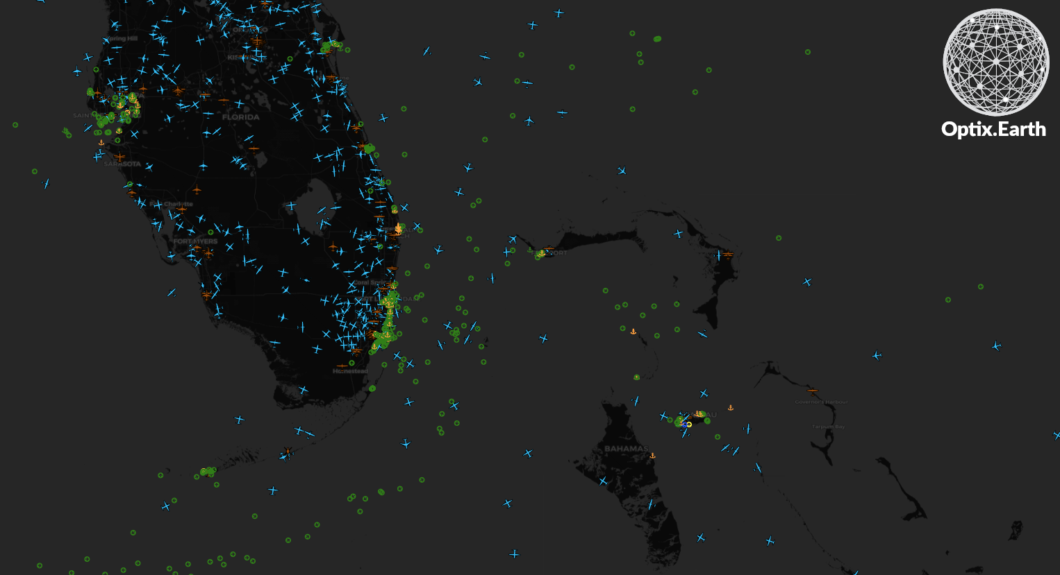
The data on these GeoMesa-Kafka topics can be serialized in a few performant formats with additional features that provide control functions over the consumer datastore. These control capabilities let us remove or update records from live layers or clear the layer entirely. This provides lots of flexibility but can make consuming or writing to these topics from analytic applications challenging or clumsy.

Kafka Streams

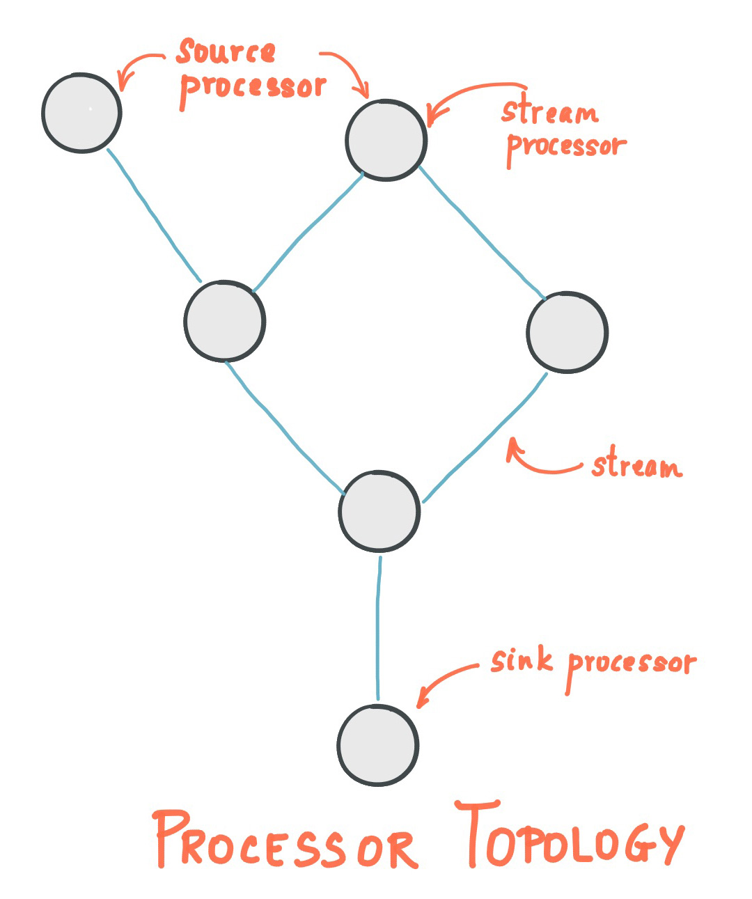
Kafka Streams is a component of Apache Kafka that enables data processing and analytics on Kafka topics. The library enables the use of higher level, SQL-like concepts to analyze streaming data. This enables simple features like filtering, aggregating or windowing streams of data as well as more complex tasks like materializing a stream into a table and joining streams or tables to each other. These functions are composed into stream topologies that are run by an application.

GeoMesa Kafka Streams Integration

Recently, GeoMesa added the ability to interoperate with Kafka Streams in a more streamlined fashion. This integration allows GeoMesa to provide the Serdes (Serializers and Deserializers) required by Kafka Streams for reading and writing data to Kafka. Additionally, GeoMesa can configure the TimestampExtractor function appropriately for the given SimpleFeatureType (SFT) and configure the correct Kafka topics for reading and writing based on the Type Name.

Below is an example of using this function, but you can run it for yourself by following the GeoMesa Quickstart Tutorial.

Streaming Proximity Example

As a motivating example, consider a stream of observations such as position updates as vehicles drive. Rendering this data as a layer in GeoServer would provide situational awareness and an overview of the state of the stream. Viewing data in this way makes it easy to imagine analytics and queries that would provide additional insight or bring attention to special events.

Say we would like to display on the map any time two entities are within close proximity. To do this, we can consume from our live feed and compare every record to all the records in close proximity, both in space and time, to find proximity events. However, this presents a few challenges that Kafka Streams can help us solve.

First, the stream of data provides position updates for entities. The data stream does not provide a continuous line through space and time. It is subsampled, giving us discrete and instantaneous observations. Therefore, when looking for proximity events we must consider a window both spatially and temporally.

Second, as data comes in we’ll need to keep the set that falls within our window in memory. This in memory data allows us to compare, or join, new observations with all the data in our window. Depending on the density or volume of data, each new observation may have to be compared with a lot of other points. A mechanism to reduce this will save us computation and provide a way to distribute this work to other threads or even other machines.

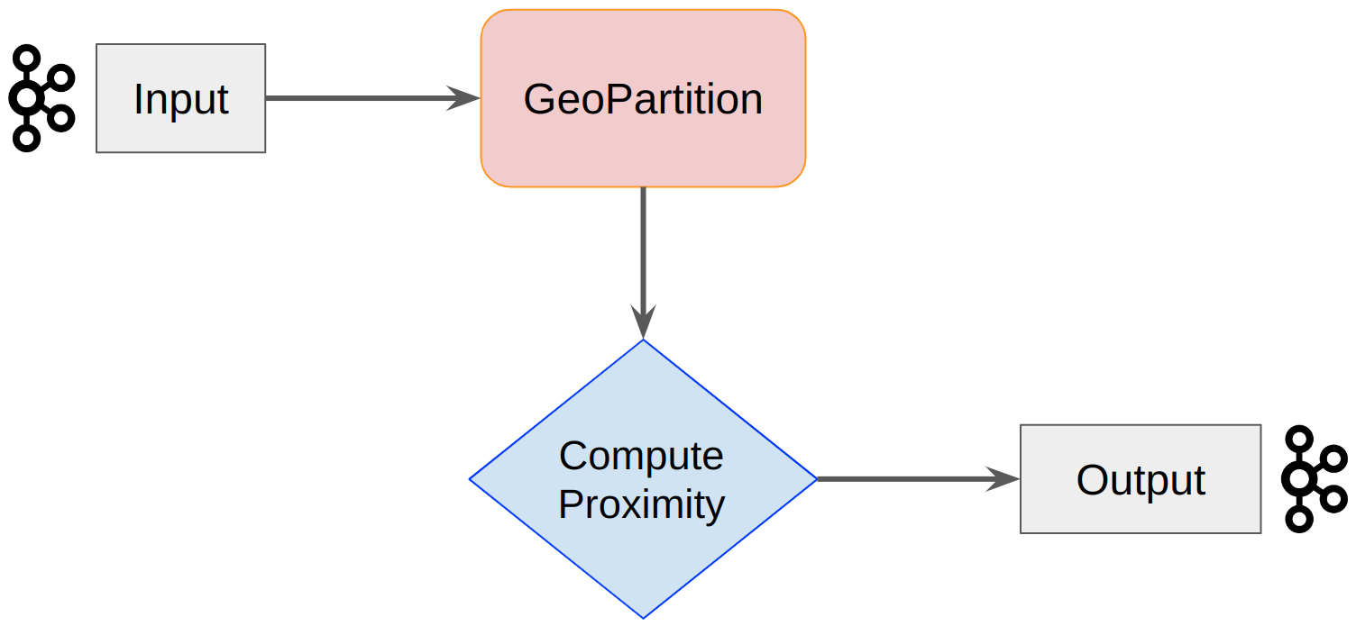
The general architecture of the process described above is to stream our input data, repartition it spatially, compute the proximity events, and stream them out.

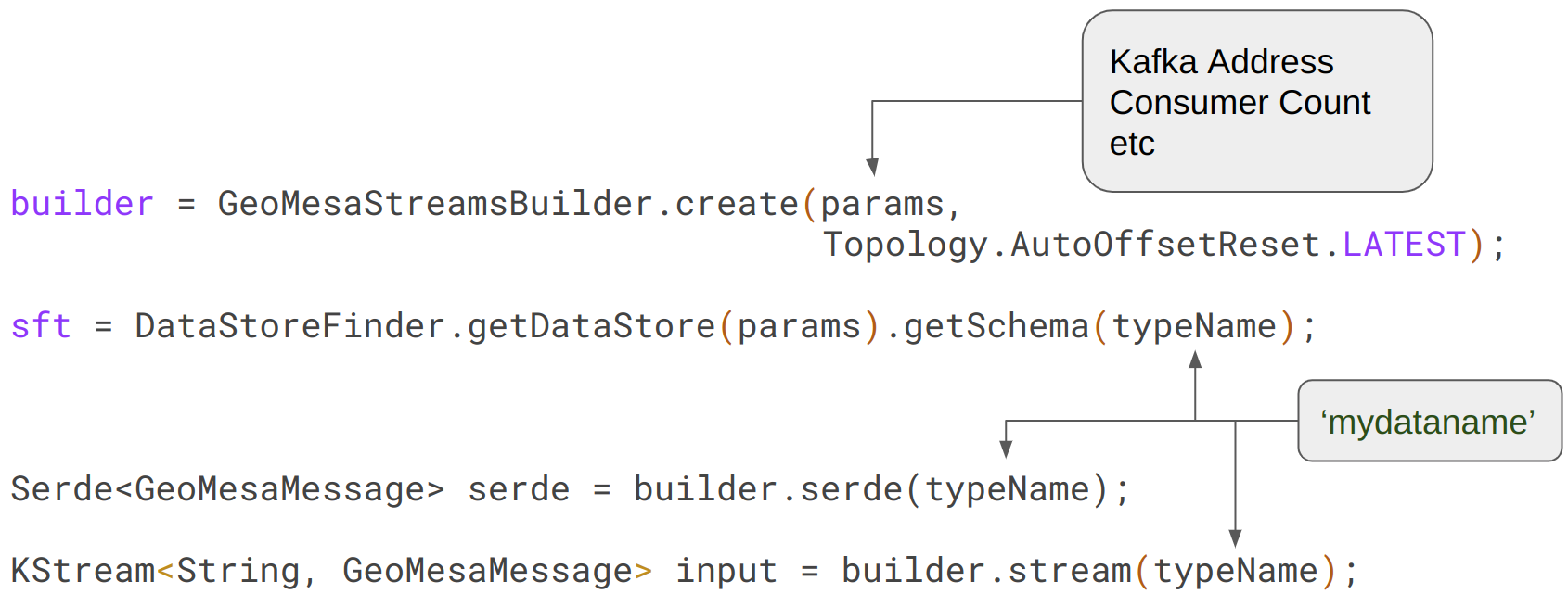
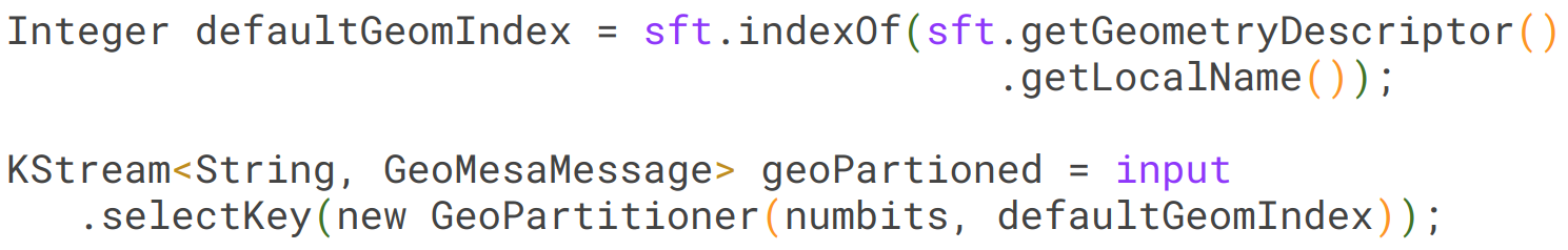
To get the input stream we can leverage GeoMesa’s new GeoMesaStreamBuilder class. This class wraps a Kafka Streams StreamBuilder class and provides serialization and deserialization (Serdes) information to Kafka Streams. This is what makes consuming GeoMesa-Kafka topics in Kakfa Streams seamless now. The GeoMesaStreamBuilder class will interpret the GeoMesaMessages and provide the record values in a List for use. Below is an example of setting up the GeoMesaStreamBuilder and retrieving the SFT. All that’s required is the GeoMesa-Kafka connection parameters and the data typeName (name of the dataset) we want to work with. We can also extract the Serdes from the builder if we need to use it in intermediate steps.

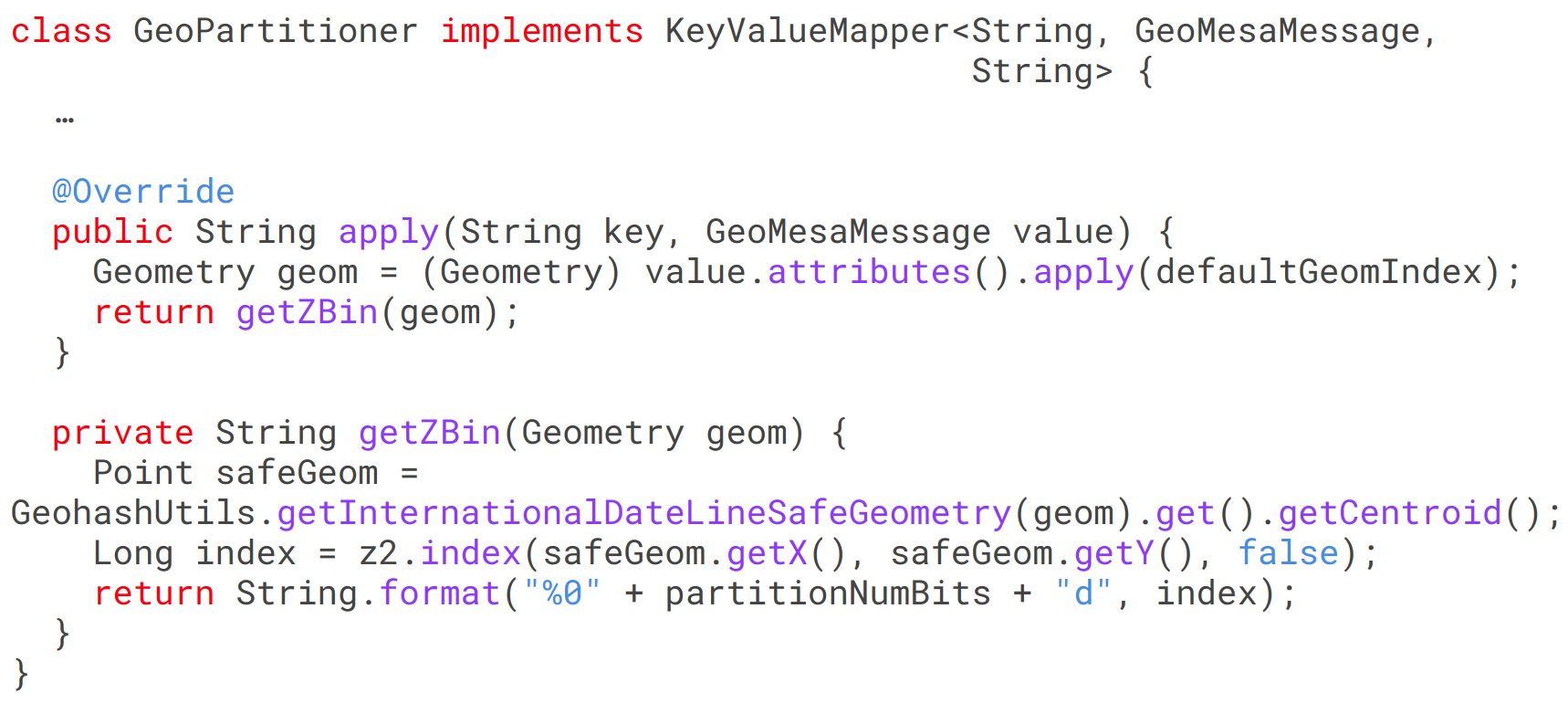
Once we have the KStream we can work on the business logic of geospatially partitioning our data and computing the proximity events. Because the GeoMesaStreamsBuilder provides our event attributes in a List we have to query the SFT to discover which index contains the spatial attribute. We then use the GeoPartitioner to select a new key for the record.

GeoMesa’s Z2 index (also known as a GeoHash) works by gridding the world into Z-Bins and organizing the bins according to their place on a Z-Order space filling curve. The GeoPartitioner example here utilizes GeoMesa’s indexing to select a Z-Bin according to the observation’s geometry. The Z-Bin ID is then used as the new key for the record. 

Having received a new key for the records, Kafka Streams will create an intermediate topic and automatically re-partition the data for us.

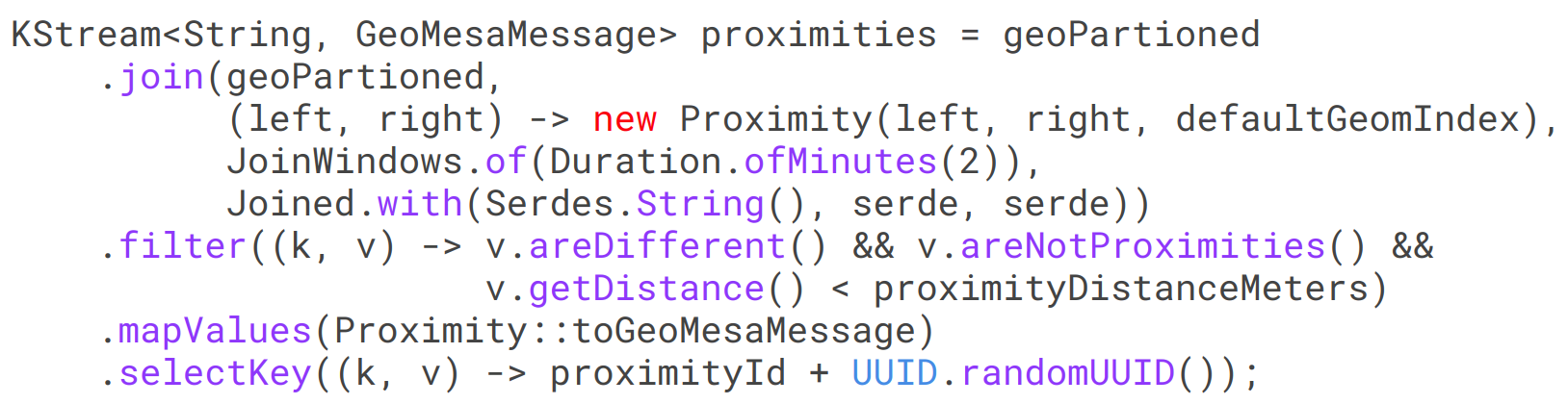
Now that our data is partitioned spatially, we can run spatial queries on it as the data is colocated. We utilize a Stream-Stream join in order to simulate a self-join on our topic. This join will join each point to every other point in its Z-Bin, thus producing a Cartesian product of the observations. Each product pair can then be compared. This is done with a Proximity class that uses GeoTools to calculate the distance.

Finally, we do some filtering to select proximities below our threshold as well as to remove points joined to themselves (from the self join) and any previous proximity events on the topic. Converting each into a GeoMesaMessage and selecting a unique key prepares the data to be written back to the source topic.

We use the same GeoMesaStreamsBuilder to write our data out, once again using the topic lookup, schema and serialize info provided by it.

Visualizing the result allows us to see the two entities traveling and the resulting proximity records produced by the pipeline.

Optix

Much of the data we handle here at GA-CCRi is geospatial in nature. We’re often looking at the behavior of aircraft, ships or other entities with geospatial coordinates. By leveraging this new capability we can create streaming geospatial analytics and data products to better understand our data streams in real time. For instance, we’re able to run real-time, global, proximity calculations for every ship in the world without having to compute every pairwise distance. This not only allows us to save on compute costs but because we’re leveraging the Kafka Streams libraries we gain their resiliency and elasticity.

For more articles or to follow or contact us, use the links below:
OPTIX | Contact us about OPTIX