Monte Carlo Pi calc

What is the first app that you code up in a new language that you are learning? I imagine most people start with the canonical "Hello World" and then move on to their own specific app. A colleague of mine always codes up the Mandelbrot set which typically involves implementing a complex number class with its associated operations - good for OO languages. For mathematical and statistical languages and APIs, I always start with Monte Carlo PI calc, a simple variant of Buffon's Needle problem. The algorithm samples n points from a unit square and then computes the ratio of points that fall within an inscribed circle of radius .5 to the total number of samples. This ratio should approach the area of the inscribed circle. Therefore, PI can be computed as the simulated ratio divided by 0.25.

To continue learning Clojure and Incanter, I implemented the algorithm as follows:

(defn mc-pi-calc [n] (/ (count (filter #(<= %1 0.5)
(map #(euclidean-distance (vec %1) [0.5 0.5])
(partition 2 (sample-uniform (* 2 n))))))
(* n 0.5 0.5)))

user=> (mc-pi-calc 10000)
3.1432

The function takes the number of samples as input and uses the sample-uniform function to generate n points in the unit square. Then, it counts the number of points that fall within a circle inscribed in the unit square using the euclidean distance function and divides this count by the total number of samples to get the area of the circle to area of the square ratio. From this, the value of PI is easily calculated.

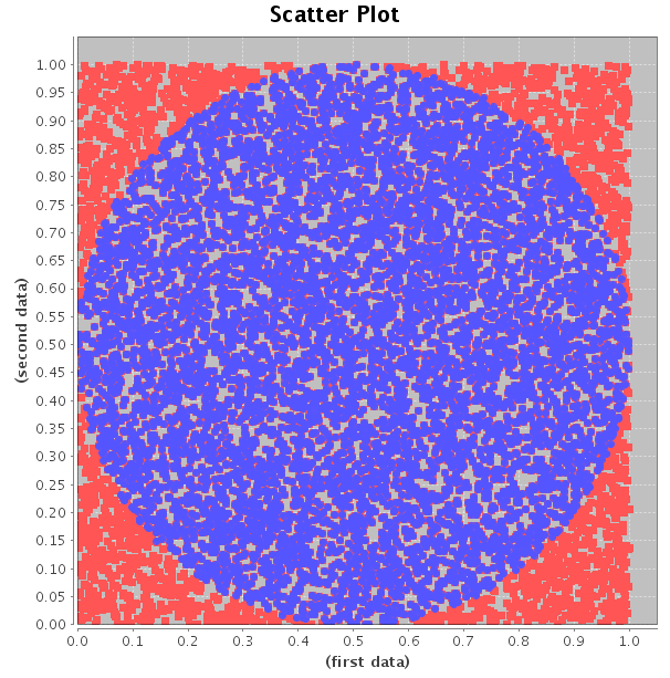
The simulation can be visualized using a scatter plot from Incanter's charts API.

;; define the sample points
(def data (trans (map vec (partition 2
(sample-uniform (* 2 10000))))))
;; plot the sample points
(def p (scatter-plot (first data) (second data)))
;; overlay the points in the circle
(def data2 (trans
(filter #(>= 0.5
(euclidean-distance %1 [0.5 0.5]))
(trans data))))
(add-points p (first data2) (rest data2))
;; view the resulting plot
(view p)

The code above produces the following chart.

The Monte Carlo Pi calc algorithm can also nicely illustrate the weak law of large numbers. Clojure's parallel processing pmap function came in handy for this task. The weak law of large numbers states that the probability that the sample average approaches the actual within some error approaches one as the number of samples approaches infinity. So, to demonstrate that, we define one sample as one computation of Pi fixing the number of random points at 100. Then, to obtain an estimate of the probability of the sample average being within an error fixed at 0.01, we take the average of 10 estimates of Pi 100 times and count the number that fell within the error. We repeat this raising the number of samples each time. The following code snippet implements the algorithm:

(def data (pmap (fn [nsamples]
(take 100 (repeatedly (fn []
(take nsamples
(repeatedly #(mc-pi-calc 100)))))))
(range 10 100 1)))
(pmap (fn [exp] (let
[d (map #(/ (sum %1) (count %1)) exp)]
(/ (count (filter #(<= (abs (- %1 3.14159)) 0.01) d))
(double (count d)))))
data)

The pmap function automatically threads the computationally intensive function over the input list using all available processors. This meant my four core laptop churned for a while on this function. The nice part of pmap is that I did not have to do anything special to get this multi-threaded functionality. And there is no reason why pmap couldn't distribute the processing across a map-reduce cluster.

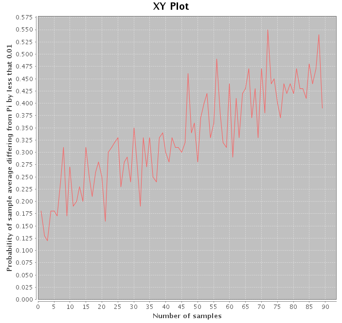
Admittedly, the MC pi calc algorithm does not converge very fast but it does illustrate the simulation capabilities of Clojure and Incanter well.

Go Back