GA-CCRi Analytical Development Services

What is an activation function?

Artificial Neural Networks (ANN) are universal function approximators with layers of feedforward computational nodes. ANNs are used in many Data Science applications involving classification and regression. However, a network with multiple layers needs those layers to be separated by nonlinear function layers, called Activation Function (AF) layers. Otherwise, the network is equivalent to a wide, single-layer, linear regression model. As computational hardware progressed and ANNs scaled to deeper networks, practitioners faced various difficulties in training the networks and developed mitigations for those issues.

What I cannot create, I do not understand.
-- Richard Feynman

To explore some of the more complex subtleties involved in activation function selection, we will set out to identify the pitfalls, list a set of requirements to avoid them, and design one or more AFs that meet those requirements.  In order to avoid reduction to the linear case,  the discussion above gives us our first requirement—(Requirement 1) Nonlinear. 

What could go wrong?

The original AF used by ANN researchers was the generic nonlinear function sigmoid.

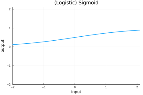
This function maps real values from (-infinity, infinity) to (0, 1). Since the output of this activation is always positive, the gradient update will be either positive for all weights or negative for all weights. This leads to an inefficient "zig-zag" approach to an optimal value. To allow for a more straightforward path to the optimum, it is desirable to have centered input data map to centered output data—(Requirement 2) Centered Output. Rather than scaling the sigmoid to get it centered, we can use the similar hyperbolic tangent tanh function.

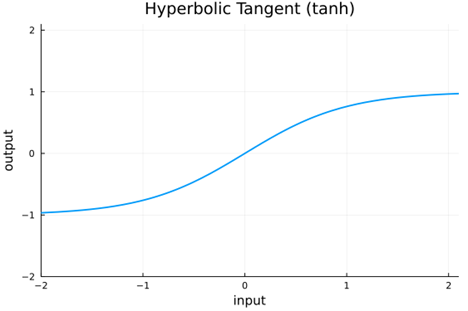
The tanh AF works, but scaling to deep networks can get sluggish because of the large number of computations. Performance also suffers when the input is far from the origin due to vanishing gradients. The tanh maps real values from (-infinity, infinity) to (-1, 1) . Practitioners sought a piecewise-linear AF to use for the nonlinear layers for speedy computation—(Requirement 3) Computationally Efficient. One prominent solution was the Rectified Linear function (relu), which is zero for negative input and the identity for positive input.

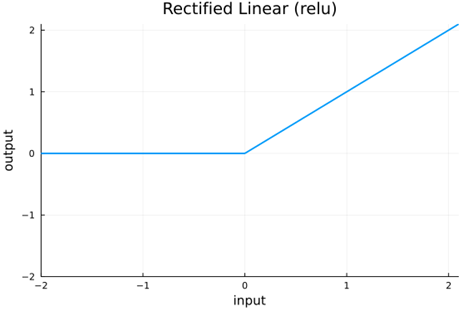
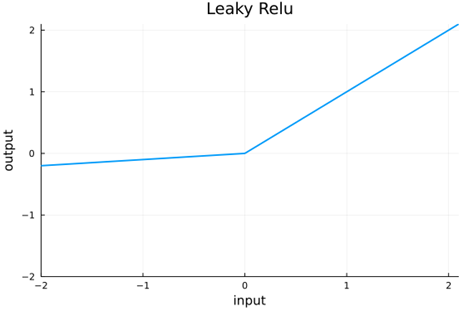
Relu allowed much deeper networks, but since all negative inputs are mapped to zero, as many as half of the nodes produce zero outputs and cannot update due to zero gradients—(Requirement 4) No Vanishing Gradients. We can avoid this by using AFs where the function is not zero except for isolated points. Leaky relu was introduced to alleviate this problem by allowing negative input to have a small slope. A related issue that is especially troublesome for recurrent networks is that of exploding gradients, which can occur when the AF has slope greater than or equal to 1 at either end of the function, i.e. the limit as x goes to infinity or -infinity.  (Requirement 5) No Exploding Gradients.

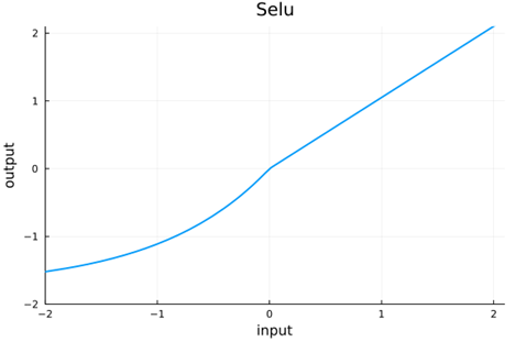
Now as networks get deeper, the value distributions can become very distorted leading to ineffective nonlinearization at best and vanishing or exploding gradients at worst. It seems prudent to provide a mechanism to keep the value distributions well-behaved. Batch normalization was introduced to do this, but some have sought for an AF to maintain normalization without such an ad hoc method—(Requirement 6) Self-normalizing. Reference [1] describes the AF selu, which is designed to maintain normalization through the first two moments—so normalized input has output with zero mean and variance is unity.

To truly maintain normalization, however, all moments above two must vanish—by definition of a normal distribution. We can take the selu idea a step further and use an anti-symmetric function to ensure that the 3rd moment—and in fact all odd moments—vanish.(Requirement 7) Anti-symmetric.

Final AF Requirements
1	Nonlinear
2	Centered Output
3	Computationally Efficient
4	No Vanishing Gradients
5	No Exploding Gradients
6	Self-normalizing
7	Anti-symmetric

With this set of requirements, we can try to construct an activation function that satisfies them and, if we are successful, test it in practice. To keep things especially simple, let's try building an AF as an anti-symmetric piecewise linear function—this will automatically satisfy Requirements 3 and 7. To satisfy Requirement 2, the function should intersect the origin. For Requirement 4, we set the slope at the origin to be greater than 1 and intersect (1, 1) and (-1, 1) to push towards a normal variance with fixed points 1 and 1. We complete the self normalization (Requirement 6) by setting the rightmost and leftmost slopes to obtain normalized output from an input normal distribution. Since the slope at either end is less than 1, Requirement 5 is also satisfied.  For reference, lets call this the Crooked "S" (crookedS) function.

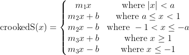
Of the parameters, we need only to choose the slope at the origin m1 and the first breakpoint a; the others are determined by the conditions for continuity and self normalization. Here we choose m1 = 1.5 and a = 0.5.

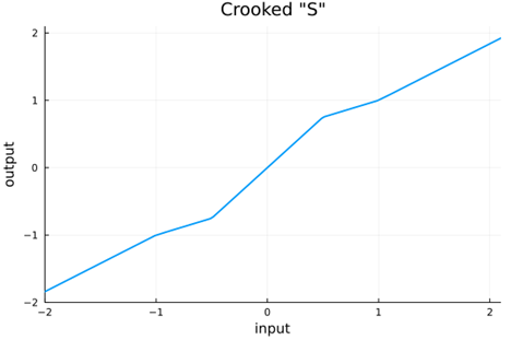
As already mentioned, crookedS has (attractive) fixed points at (1, 1) and (-1, -1), meaning that running any given value through the function iteratively will converge to 1 or -1 depending on if it is positive or negative. We can get more fixed points in the hope of making things more robust by crossing the line y = x multiple times. Rather than introducing more breaks in crookedS, we can use a sinusoid as follows, again setting the slopes at either end to ensure self normalization.

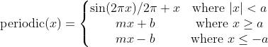
To ensure a normalizing and differentiable function, we must have m = 0.683761, a = 1.30121, and b =0.411493 .

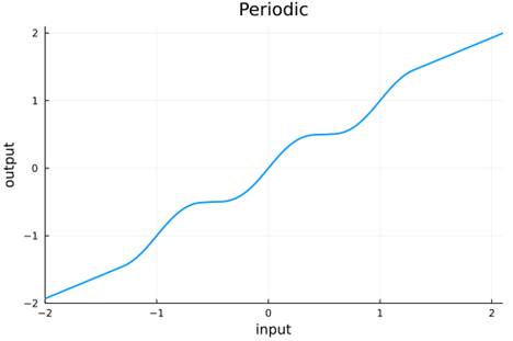
Table of requirements and activations

Requirement	Sigmoid	tanh	relu	Leaky relu	selu	crookedS	periodic
1. Nonlinear	x	x	x	x	x	x	x
2. Centered Output		x	x	x	x	x	x
3 . Computationally Efficient		?	x	x	?	x	?
4. No Vanishing Gradients				x	x	x	x
5. No Exploding Gradients	x	x	?	?	?	x	x
6. Self Normalizing					x	x	x
7. Anti-symmetric		x				x	x

How well do these activations normalize a network?

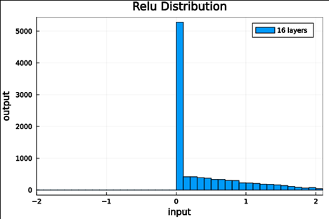
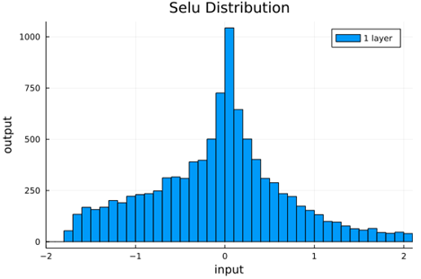
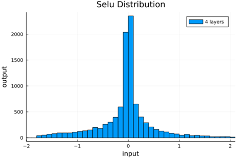
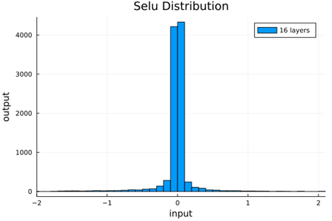
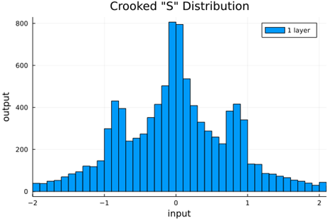
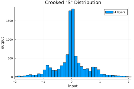
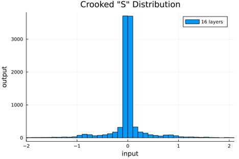
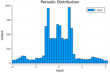
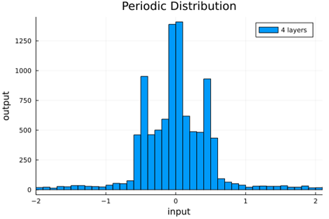
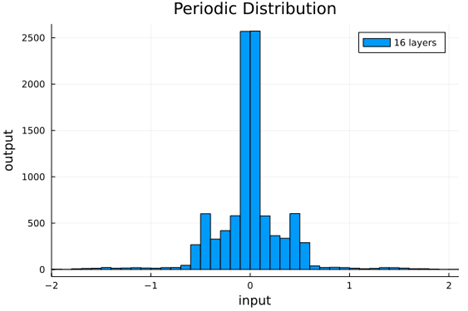
We should check to verify that the self normalizing AFs (selu, crookedS, and periodic) actually maintain normalization over several layers.

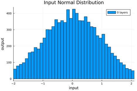
Now we run the samples through consecutive layers of the activation functions.

Unweighted Layers	1 Layer	4 Layers	16 Layers
relu
selu
crookedS
periodic

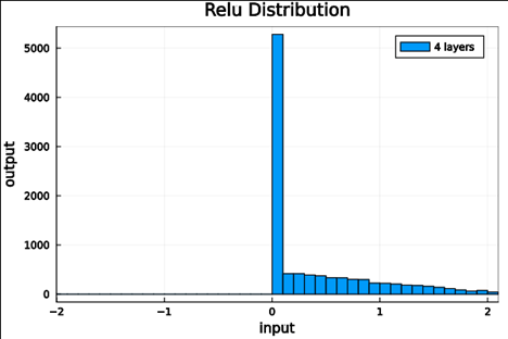
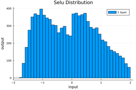
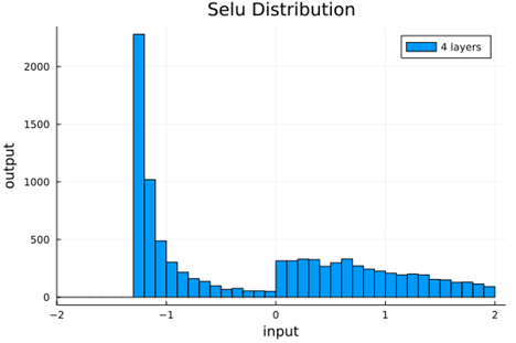
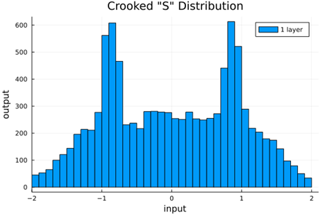
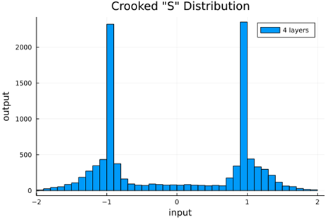
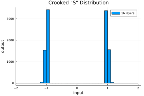
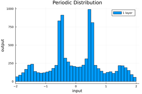
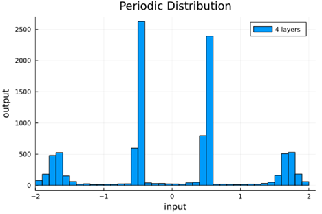
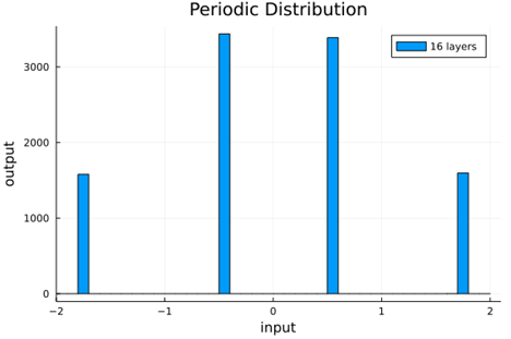
From this we can see how the distributions propagated through the proposed activations (crookedS, periodic) converge to fixed points in proportions that have zero mean and variance of 1.0. For a more realistic look at the distributions in practice, we populate the weights with values from a normal distribution and compute the outputs of a forward model run before any training occurs.

Normal Weights	1 Layer	4 Layers	16 Layers	Variance (after 16 layers)
relu				< 5e-7
selu				0.075 ± 0.005
crookedS				0.22 ± 0.03
periodic				0.16 ± 0.01

 

Put it to the test

To rapidly test these ideas, we use a convolutional network to classify the CIFAR-10 images [2] into 10 classes. Here we have chosen the simple architecture SimpleNet [3] (a great read for tips on developing simple yet robust CNNs). The architecture is shown in the figure below.

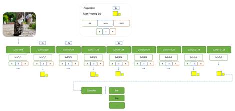
SimpleNet has 13 convolutional layers followed by a fully-connected Multi-Layer Perceptron (MLP) classifier. For our baseline test, we train this network (referred to here as BatchNorm) with three fully-connected layers followed by the output layer. We train without data augmentation for 100 epochs using the Adam optimizer with learning rate 1e-4 for the first 79 epochs, and dropping to the learning rate 1e-5 starting with the 80th epoch. All images are normalized in preprocessing. The baseline training achieved a top-5 accuracy of 86.9% with 33 seconds per epoch on my NVIDIA Titan X GPU hardware. To test the self-normalizing AFs (and remove the BatchNorm layers), we must take care not to introduce distortions at any layer. So for the self-normalizing networks (SNNs), in addition to removing the BatchNorm layers, we replace the MaxPool layers with MeanPool and follow by doubling the output. We also need to initialize the weights with the Kaiming Normal method. Since we are using dropouts to help with generalization, we use the normalizing AlphaDropout layers in place of the usual Dropout layers. Training the network with the crookedS AF resulted in training time of just 27 seconds per epoch—nearly a 20% speedup from baseline—showing the computational benefit from removing BatchNorm layers. However, the top-5 accuracy was a dismal 64.3%.

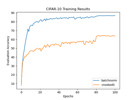
Perhaps this is simply the penalty for getting rid of BatchNorm? No. Testing with the selu AF yields similar computational speed with the respectable top-5 accuracy of 85.6%. Nonetheless, a quick test on the MNIST dataset using a MLP suggests that the fully connected classifier is not the problem for crookedS. What would happen if we use selu for the convolutional part and crookedS for the fully connected classifier? Surprisingly, this results in faster convergence and even better top-5 accuracy (86.6%) than selu alone! Furthermore, if we train again with selu in the convolutional part but the periodic AF in the classifier, the top-5 accuracy is 87.1%—a trifle better than baseline.

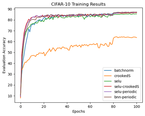
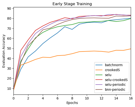
Looking just at the first 16 training epochs, we see that the use of the proposed activations in the fully connected classifier enhance the convergence rate to top evaluation accuracy compared to baseline (BatchNorm) and selu.

	Top-5 Accuracy	Train Time per Epoch (s)	Speedup (over baseline)
batchnorm	86.9%	33	--
crookedS	64.3%	27	18%
selu	85.6%	27	18%
selu-crookedS	86.6%	27	18%
selu-periodic	87.1%	27	18%
bnn-periodic	87.2%	31	6%

Conclusions

Through this exercise, we found that we could build some simple Activation Functions by compiling a set of requirements to avoid some of the problems that have plagued previous implementations and ensuring those AFs satisfy the requirements. We arrived at two functions, Crooked "S" and a periodic function, that checked all the boxes, and we tested those against our baseline using the SimpleNet architecture on the CIFAR-10 data. The two proposed AFs performed poorly when used for the convolutional part of the network, but matched or exceeded baseline accuracy when used just for the fully connected classifier layers. Eliminating batch normalization layers via self-normalizing activations allowed for a nearly 20% speedup. Further, our testing suggests training convergence is enhanced.

Based on these observations, it would be great to see an analysis with the proposed activations on deep feed forward networks and recurrent neural networks, where the advantages of the self normalizing property may really shine. A deep-dive into the failure of the AFs in the convolutional part of the network would also be enlightening. We may speculate that the correlations introduced with convolutions may distort the distributions to an extent such that the self-normalizing property is ineffective.

References

[1] Klambauer, G., Unterthiner, T.,  Mayr, A., and Hochreiter, S., Self-Normalizing Neural Networks, 2017, https://arxiv.org/abs/1706.02515
[2] Krizhevsky, A., Learning Multiple Layers of Features from Tiny Images, 2009, https://www.cs.toronto.edu/~kriz/learning-features-2009-TR.pdf
[3] Hasanpour, S. H., Rouhani, M., Fayyaz, M., and Sabokrou, M., Lets keep it simple, Using simple architectures to outperform deeper and more complex architectures, 2016, https://arxiv.org/abs/1608.06037