GA-CCRi Analytical Development Services

According to the Wikipedia page for the game Battleship, the Milton Bradley board game has been around since 1967, but it has roots in games dating back to the early 20th century. Ten years after that initial release, Milton Bradley released a computerized version, and  now there are numerous online versions that you can play and open source versions that you can download and run yourself.

At GA-CCRi, we recently built on an open source version to train deep learning neural networks with data from GA-CCRi employees playing Battleship against each other. Over time, the automated Battleship-playing agent did better and better, developing strategies to improve its play from game to game.

Current progress has been made to establish a framework for (1) playing Battleship from random (or user-defined) ship placement (2) deep reinforcement learning from a Deep Q-learner trained from self-play on games starting from randomly positioned ships and (3) collecting data from two-player Battleship games. Our experiments focused on how to use the data collected from human players to refine the agent’s ability to play (and win!) against human players.

Q-learning

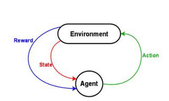
There are various technical approaches to deep reinforcement learning, where the idea is to learn a policy that maximizes long-term reward represented numerically. The learning agent learns by interacting with the environment and then figures out how to best map states to actions. The typical setup involves an environment, an agent, states, and rewards.

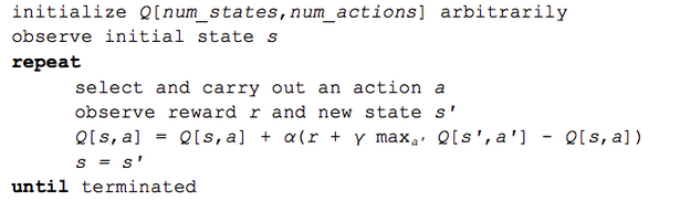
Perhaps the most common technical approach is Q-learning. Here, our neural network acts as a function approximator for a function Q, where Q(state, action) returns a long-term value of the action given the current state. The simplest way to use an agent trained from Q-learning is to pick the action that has the maximum Q-value. The Q represents the “quality” of some move given a specific state; the following pseudo-code outlines the algorithm:

In practice, when we are training the Q-learner, we do not always pick the action that has the maximum Q-value as the next move during the self-play phase. Instead, there are various  exploration-exploitation methods designed to balance the ‘exploring’ of the state space in order to gain and access information on a wider range of actions and Q-values versus ‘exploiting’ what the model has already learned. One basic method is to start with completely random choices some percentage of the time and to then slowly decay to a smaller percentage as the model learns. Playing Battleship, we found that starting at 80% and decaying to 10% worked well.

More Advanced Deep Q-learning Methods

To help with faster training and model stability, more advanced deep Q-learning methods use techniques such as experience replay and double Q-learning. Experience replay is when games are stored in a cyclical memory buffer so that we can train batches of moves and we can sample from games that were already played. This helps the model avoid converging to a local minima because the model won’t be getting information from a sequence of moves in a single game. It also helps the model take into account past moves and positions, providing a richer source of training. Double Q-learning essentially uses two Q-learners: one to pick the action and another to assign the Q-value. This helps to minimize overestimation of Q-values.

To generate the sample data, we began with the open source phoenix-battleship, which was written in elixir using the phoenix framework. We modified phoenix-battleship to save logs of ship locations and player moves and we made slight configuration changes for the sizes of ships and generated data. We hosted the app on Heroku, encouraged our co-workers at GA-CCRi to play,and saved logs of the games that were played using the add-on papertrail. We collected data from 83 real, two-person games.

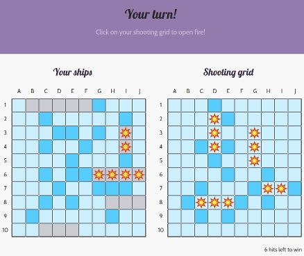
The following shows one GA-CCRi employee’s view of a game in progress with another employee. Dark blue squares show misses, the little explosions show hits, and the gray squares on the left show where that player’s ships are.

We wrote the code in PyTorch with guidance from the Reinforcement Learning (DQN) tutorial on pytorch.org as well as Practical PyTorch: Playing GridWorld with Reinforcement Learning and&nbsp Deep reinforcement learning, battleship.

We trained an agent to learn where to take actions on the 10 by 10 board. It successfully learned how to hunt for locations and target the squares around a hit to sink the rest of the ship once one part of it has been found. Next, we plan to refine the agent using the collected data to perform better than human players.

Ship Placements for Collected Game Data

Heat maps of the ship locations show that there are clearly favored positions for the ships. In particular, players favored rows B and I and columns 2,4, and 9. We can also see that players often tried to hide the size 2 ships in the corners.

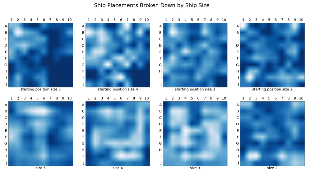
“Starting position”  refers to the square that is the upper left most position on the ship. From the starting position the ship has two possible placements: going horizontally to the left or going vertical and down.

Model Evaluation

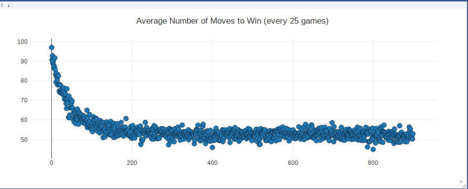
The graph above is a scatterplot of the average number of moves it took for one player to win, calculated over the most recent 25 games, as the agent was training.

We used a basic Deep Q-learning reinforcement method to train a learning agent. Ship placements were randomly initiated to start each game, and then the games were played out using the learning agent. Initially, 80% of the moves were random to encourage the model to explore the possible move and hit locations; gradually we relied more on the model to pick the next move based on what it had learned from previous games.

At the end of training, the learning agent averaged around 52 moves to win each game. At this point our model has learned a method better than the hunt/target method (randomly shoot squares and then if a square is selected shoot the squares around it). The benchmark distribution for that strategy averages around 65 moves. But, it has not yet been able to have shorter game playing time than a probability-based method which, rather than randomly shooting squares, first selects squares with ‘higher likelihood’ (based on the total number of configurations that cover that square) of being shot to hit. The benchmark distribution for this strategy averages around 40-45 moves.

Game Play Strategies the Model Learned from Training

We watched the agent play out a few games to assess if it had learned any strategies and what those strategies were.

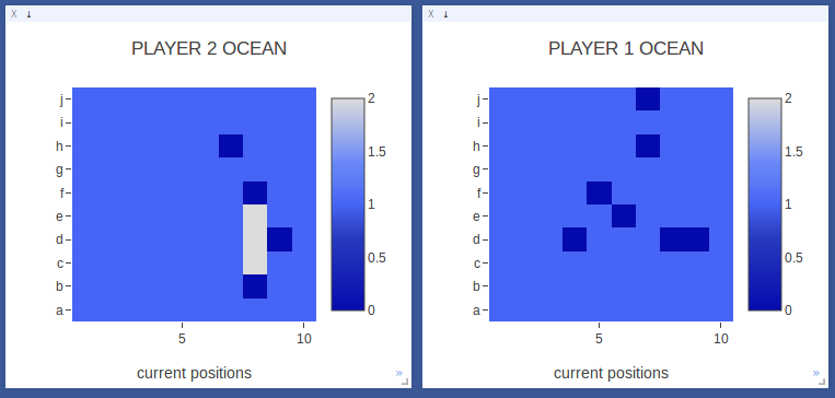
The play board is visualized as an ‘ocean’ where light blue represents unsearched squares. As the game is played, dark blue squares represent squares that have been searched but are misses (no ship) and white squares represent squares that are hits (a ship has been hit).

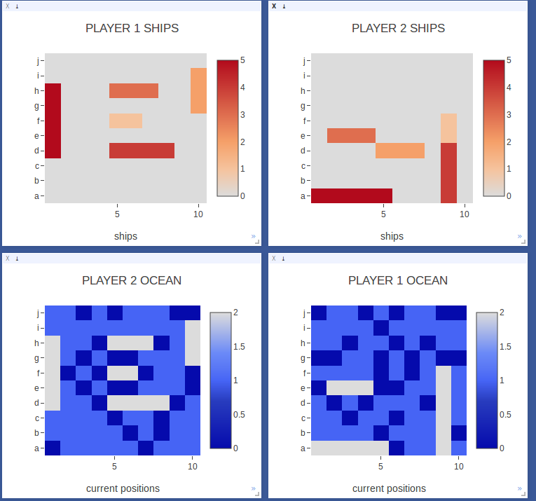
As you can see even from the single frame (and which is more obvious when you watch a game unfold), the agent did indeed learn some strategies.

• Once a ship has been hit, the agent continues to target squares around that hit. After a size 5 ship, the agent does not always continue targeting squares around it; see player 2’s play for an excellent example. This is effective, since 5 is the largest size.
• The agent searches for ships using a diagonal or modified parity method. This makes sense because searching along adjacent diagonal squares but not adjacent squares covers more ground to hit a ship given that they are size 2, 3, 3, 4, 5.

Watching a Sample Game using the Agent

Boards	Moves
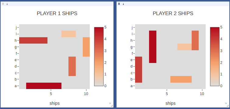	Starting Ship Positions for ships of size 5,4,3,3,2.
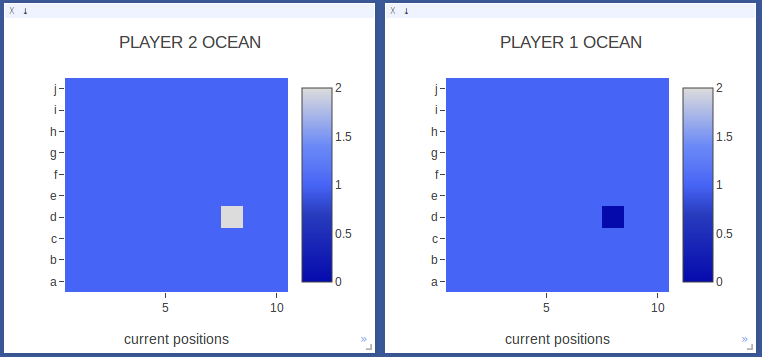	In move 1, Player 2 hit a ship!
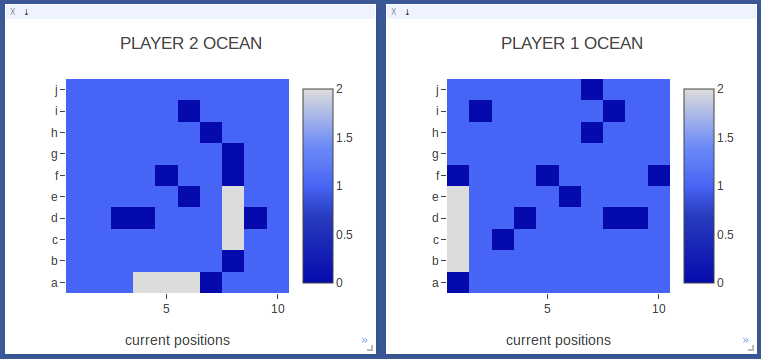
	Now Player 2 starts searching the squares around the first hit. Player 1 starts exploring another area of the board.
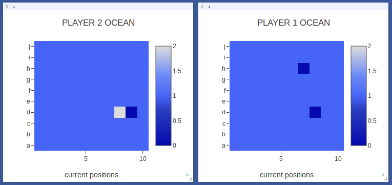
	Player 2 sinks the first ship! In moves 3-6 Player 2 aimed hits around the initial hit and found the bounds on either side. The model understands how to hunt for the rest of a ship once it gets a hit.
	After sinking its first ship, Player 2 starts exploring another area of the board. Notably, it does not keep trying to continue to find hits around the ship it already sunk. The model has some understanding that a ship has been sunk.
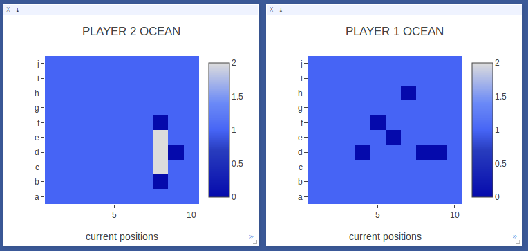
	Player 1 finally sinks its first ship! In moves 8-18, Player 1 continues searching the board along different rows and columns. Note that the diagonal is along the main diagonal, where ships have a higher probability of being placed. The model has a non-random search strategy.
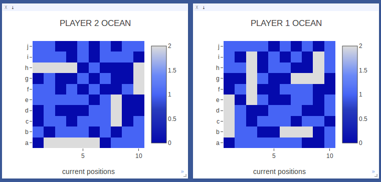	Player 1 wins! Even though Player 1 took more moves to sink its first ship, Player 2 had trouble finding the last size 2 ship in the end.