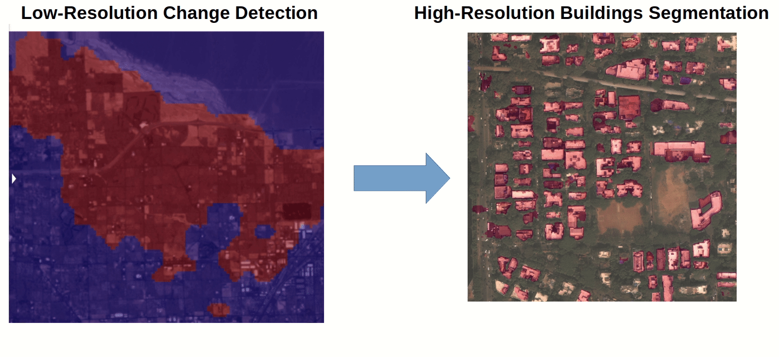
Coarse Earth Change Detection: Supervised and Self-Supervised training
Change detection from aerial or satellite images is in great demand for monitoring various activities. The detection of wide area change over the past year has garnered a lot of interest, with a wave of publications using different methodologies and different data sources to solve the task [1,2]. In this blog post we will focus only on multi-spectral images, but there is a great deal of literature on training a model with a variety of data sources, such as SAR, optical, multi-spectral, hyper-spectral, heterogeneous, and aerial. Different techniques have been developed to solve the change detection task in a wide range of applications, including urban development, future planning, environmental monitoring, agricultural expansion, disaster assessment, and map review. We want to train a model that detects areas of larger artificial change, such as the construction of new housing developments or infrastructure, and not smaller changes such as the movement of cars or natural changes due to seasonality or weather conditions.
In this post, we will show how we have implemented a small model that runs on a coarse or low-resolution image to identify modified areas. This can be thought of as a setup step for a more accurate and complex analysis that can be performed on the highlighted areas.
Supervised Training
Let's look at a way to train a neural network using a collection of clean, ready-to-use images with annotations that tell us which image pixels have changed from a previous version. Onera Satellite Change Detection [6] is a dataset published by the French aeronautics, space and defense research laboratory Onera.
Data
The Onera dataset is composed of 24 multi-spectral images taken by Sentinel-2 satellites between 2015 and 2018. Locations are collected in Brazil, USA, Europe, the Middle East and Asia. For each location, Sentinel-2 obtained pairs of 13-band multi-spectral satellite images. Pixels are annotated by focusing on urban changes, such as new buildings or new roads, and ignoring natural changes such as seasonality, vegetation growth, and tides. The annotation for each image is man-made and is a binary pixel mask composed by 1 and 0 respectively if that area has changed from the previous image. This is the ground truth that will tell us the true label for each pixel during training.
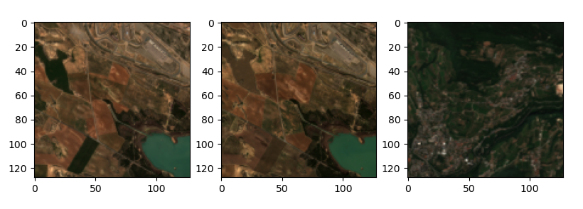
Original ground truth mask with GSD 10m |
|
|
|
Training
Now that we have a binary label, we can train a model based on the Resnet architecture pre-trained on Imagenet. Since we have well-aligned images and annotations, we can use a technique called Early Fusion [7] in which the input to the network is composed by the oldest image concatenated in the channel dimension with the recent one. The implemented modified model has a multi-spectral input image of 4 or 6 bands, which in the Early Fusion configuration corresponds in doubling to 8 or 12 the input channels.
|
Sentinel Bands |
| 4 bands model | B2(B),B3(G),B4(R),B8(NIR) |
6 bands model |
B2(B),B3(G),B4(R),B8(NIR),B11(SWIR1),B12(SWIR2) |
Here we see a comparison between 4 and 6 band input, along with the (coarse) output of the trained resnet models.
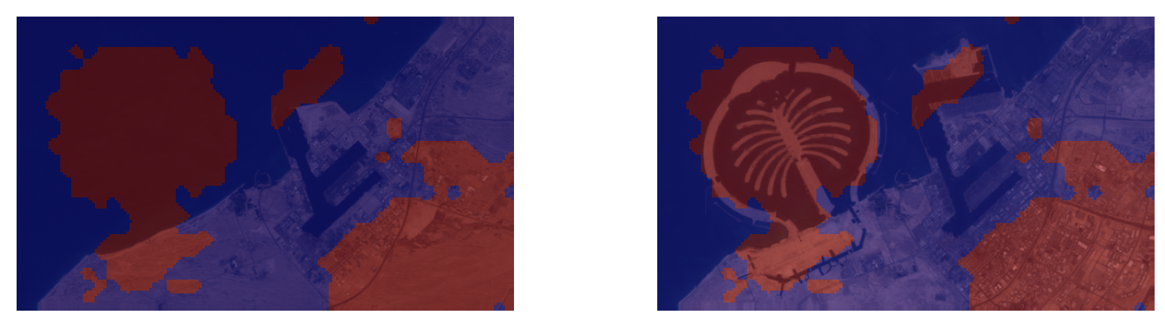
| Dubai | |
| Before | After |
 |
 |
| Resnet 4 band | Resnet 6 band |
 |
 |
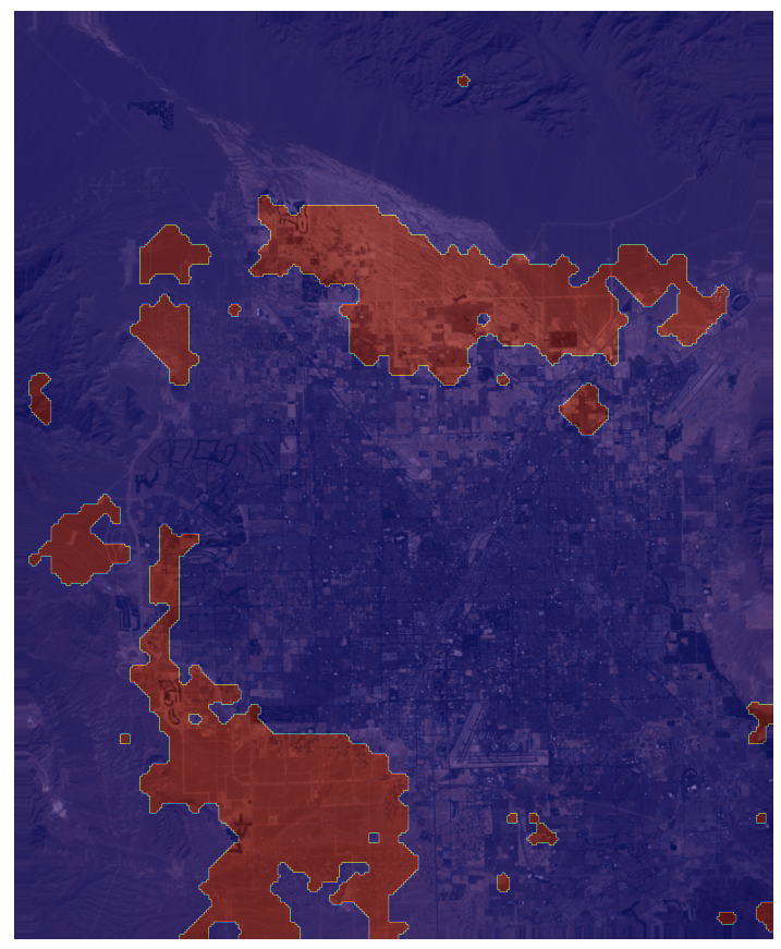
| Las Vegas | |
| Resnet 6 band | |
 |
 |
| Resnet 4 band | Resnet 6 band |
 |
 |
The model implemented has best performance using 6 band inputs instead of 4. Below is the Top-1 accuracy of the trained models on the validation set (split from Onera dataset).
Architecture |
Bands |
Validation Accuracy [%] |
Resnet50 |
4 |
88.95 |
6 |
90.07 |
In this first example, we see how a dataset created only for change detection can be used to train a neural network in a supervised way. Despite the average good performance given the small amount of data, we can see that annotating each pixel of an image is not a scalable practice to the large amount of data available from satellites.
Self-Supervised Training
Why train with more degrees of freedom? What advantages would it bring for data mining? Can we get a better result with less effort, without labeling any satellite image? The change detection model may require even more data to better generalize about artificial and natural changes in the real world image. We can train these models in a self-supervised or unsupervised way; this can really be a game changer given the amount of data available for free from many satellite missions.
Loss Function and Architecture
First we need to define a loss function and the model architecture that we will use during training. Then we can examine the data and see how to frame the problem.
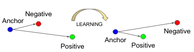
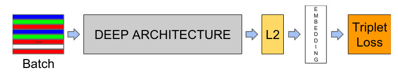
The loss function is the criterion that we will use to estimate the error that the model is committing by predicting one of the possible outcomes. It is a positive value and will be as large as the error committed. Ranking losses are a type of loss function, different for the one used in the session before, in which instead of predicting a value or class given an input (like for Cross-Entropy Loss or Mean Square Error Loss) they want to predict a similarity or distance between the inputs. This is why it is also called metric learning. To use triplet loss, which is a ranking loss, we first extract the embedded representation of the input images, and then we measure the Euclidean distance between these two instances to see if they are similar. Note that here we are not even interested in the values of each representation, but only in the distance between them, which can be encoded in the changed / not-changed binary classification. This type of loss used with a Siamesian neural network architecture offers a configuration that allows for very flexible input data. Triplet loss [8] is defined for triplets of chips that represent an anchor, positive and negative example.| Anchor | Positive | Anchor | Negative |
 |
 |
|
 |
During training, we want to learn characteristics that push the anchor away from the negative example and keep the anchor close to the positive example.
Triplet loss |
|
To do so, we need to select or mine the triplets output from the model at each iteration and learn just from the selected triplets, so we will only select semi-hard negatives. This means that from each batch of triplets that we pass through the model, we will select only the ones that have a representation vector distance between the two pairs (Anchor-Positive and Anchor-Negative) within a fixed margin.
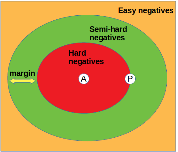
The condition that defines a semi-hard negative triplet during mining is:

The first term in the subtraction represents the distance between the anchor and the negative i-th example, and the second term is the distance between the anchor and the positive. This triplet mining is essential for training success because it gives us a criterion for filtering triplets that are generated with incorrect conceptual formulation. However, for this type of training we must consider some noise in the label because the mining algorithm will filter most but not all the incorrect triplets.
The architecture of a Siamese neural network with shared weights is followed by the L2 normalization that we can visualize in the diagram below. The Siamese neural network is just a model with shared weights. This model will be used to calculate the representation for each chip of the triplet. L2 normalization is needed to have a relative comparison between vectors before calculating the Euclidean distance, so we can more easily define a threshold for the modified and unmodified areas.
To frame the earth change detection we can use the geographical information of the data with the triplet loss concept. We can approximate the labels of the data by considering that images taken from distant places should look different, and an image from the same location over a different time period should look very similar. Let's take a look at clean data from a dataset that has been curated for a different purpose and see how it fits into change detection training.
Dataset
The Earth Net 2021 dataset [6] is a collection of ready-to-use Sentinel-2 images of 128x128 chips with no clouds or missing data. This is critical because this data is ready to use and not like raw data, which can introduce many other variables. The following table shows selected bands used during training.
Name |
Available GSD |
Wavelength |
Description |
B2 |
(10m),(20m),(60m) |
496.6nm (S2A) / 492.1nm (S2B) |
Blue |
B3 |
(10m),(20m),(60m) |
560nm (S2A) / 559nm (S2B) |
Green |
B4 |
(10m),(20m),(60m) |
664.5nm (S2A) / 665nm (S2B) |
Red |
B8 |
(10m) |
835.1nm (S2A) / 833nm (S2B) |
NIR |
Here are some examples [11] of how the compositions of these bands can highlight aspects of nature from the radiation reflected in that spectral band [12].
This EarthNet2021 dataset was proposed to predict seasonal weather, but let's see how we can use it to solve our task. After splitting the dataset into training and test groups, the training group contains 30,000 samples or data cubes from different locations in Europe. Each of these cubes contains 30 images 5 frames per day (128 × 128 pixels or 2.56 × 2.56km, GSD 20m ) with four channels (blue, green, red, near infrared) of satellite images from November 2016 to May 2020.
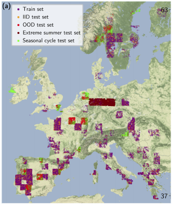
This dataset was designed to look only for natural features, so there is poor urban content in the images. Another aspect to note is that all crops come from Europe, so there won't be much variability in the natural context.
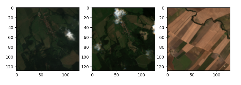
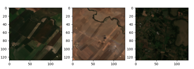
Triplets mining
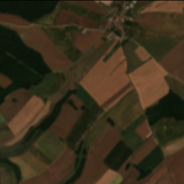
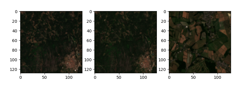
Let's see the triplets generated using two randomly selected data cubes from two different locations. The first data cube will be used to select the anchor and the positive and the second data cube will be used to select the negative chip. We can see how the anchor and the positive will translate into two perfectly aligned crops of the same location in a different time frame, which have a lot in common and highlight the change in vegetation given by seasonality and weather conditions.
Triplets generated for Self Supervised training
Test
The test is done on Landsat7 satellite 8-bit images from ETM+ (Enhanced Thematic Mapper Plus) sensor that collects data from 1999 to the present.
Name |
GSD |
Wavelength |
Description |
B1 |
(30m) |
0.45 - 0.52 µm |
Blue |
B2 |
(30m) |
0.52 - 0.60 µm |
Green |
B3 |
(30m) |
0.63 - 0.69 µm |
Red |
B4 |
(30m) |
0.77 - 0.90 µm |
Near-IR |
The first step we have to do before running the inference is to align the two images from the same location in a different time frame. Then, we run them through the model and compute the Euclidean distance between each vector for each pixel.
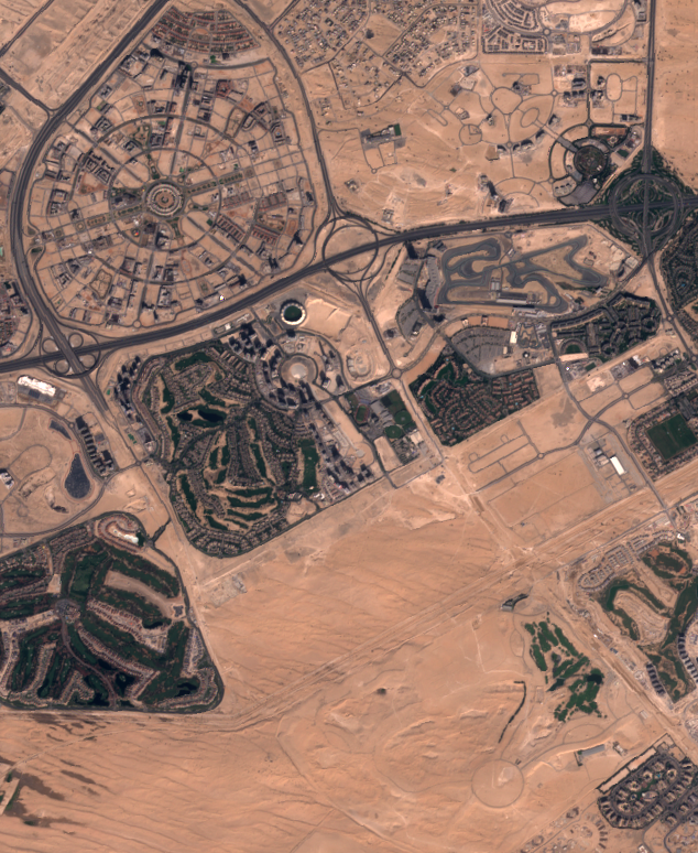
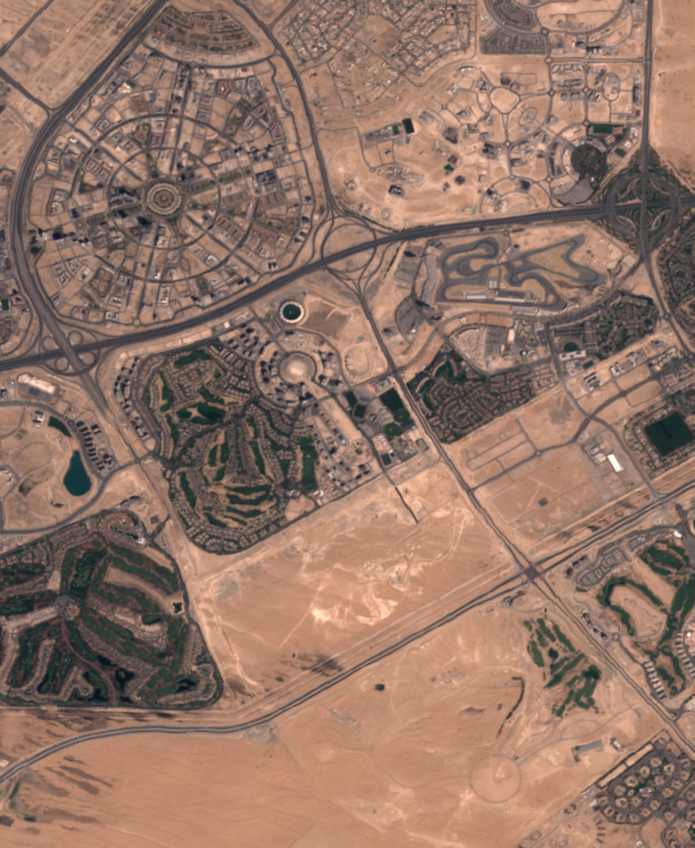
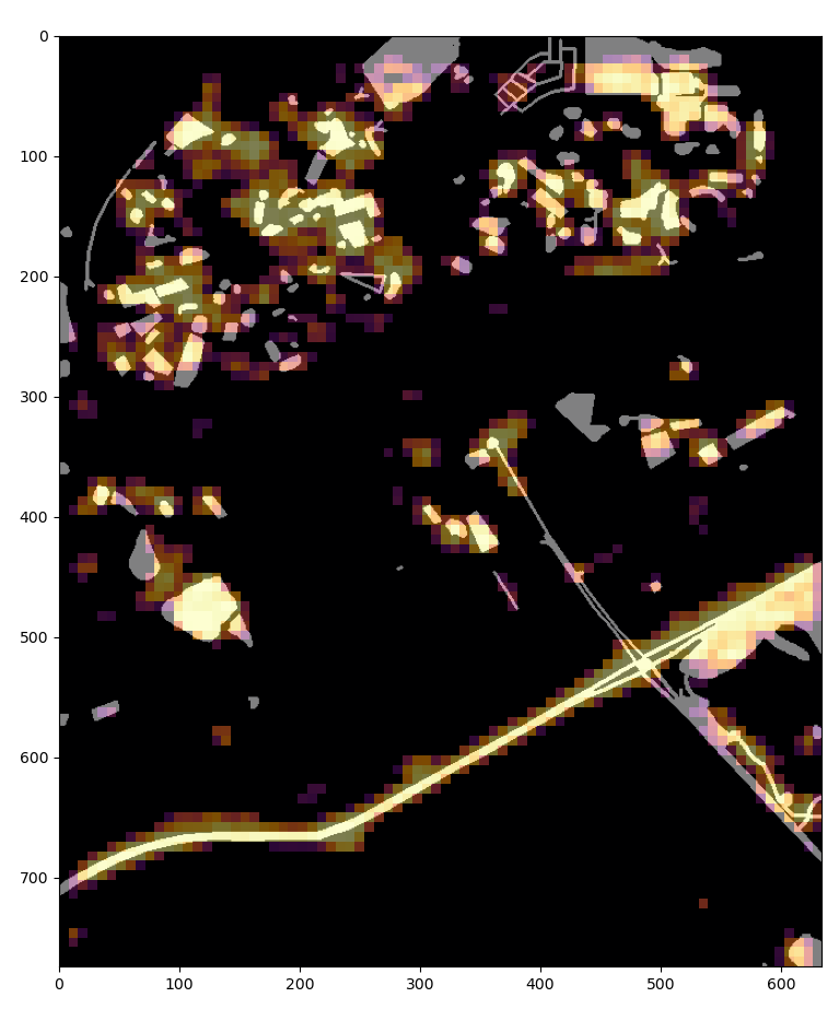
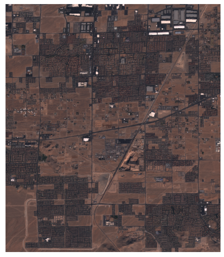
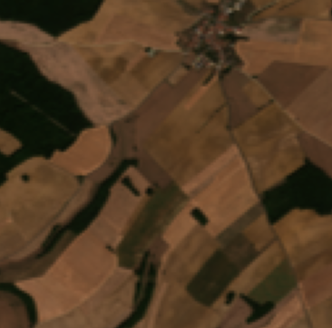
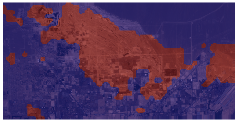
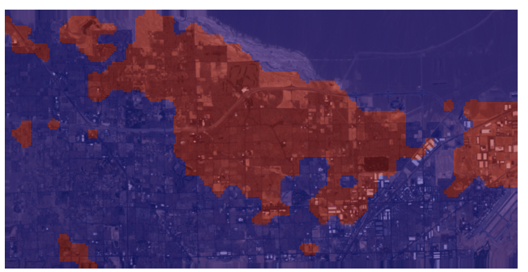
Dubai (1999 - 2020)
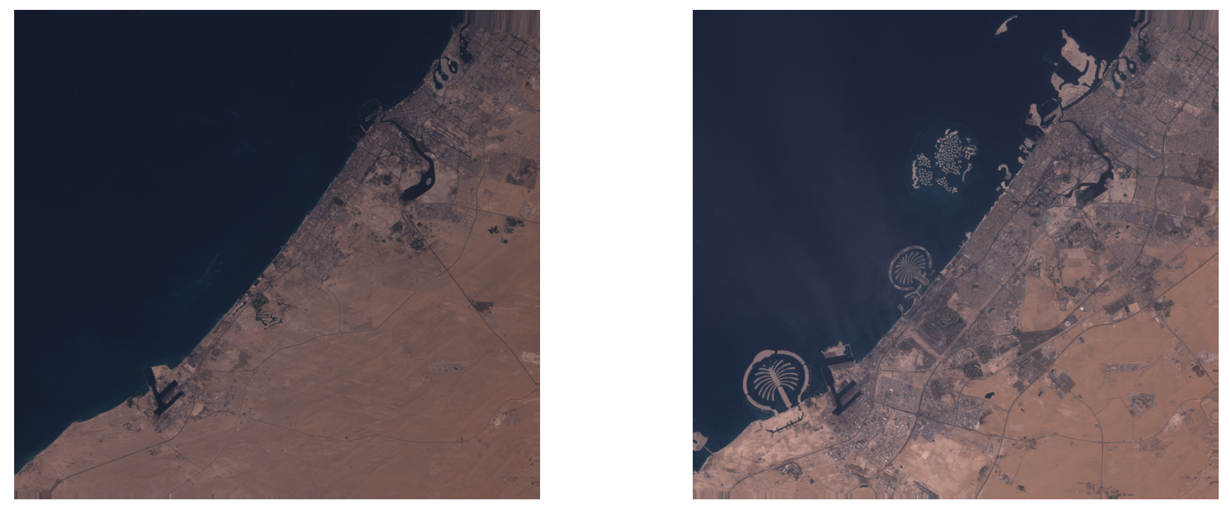

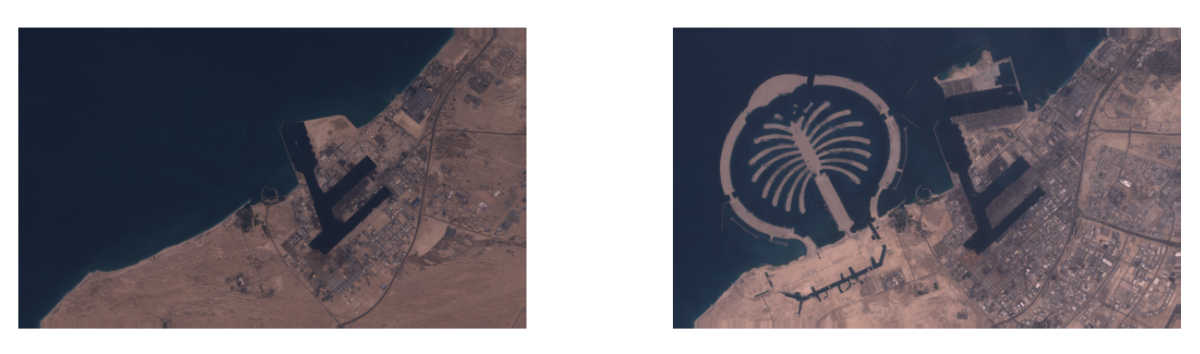
As we can see from the heatmap overlay on the image, the threshold part highlights where the biggest changes have occurred, with more emphasis in the brighter parts. Let's threshold the model outputs and look at a more detailed region of interest:
Detail of Dubai 1999 - 2020
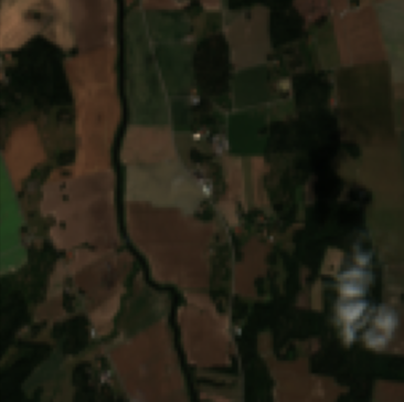
Next, another example on Las Vegas.
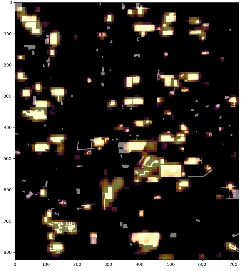
Las Vegas 1999 - 2020

 |
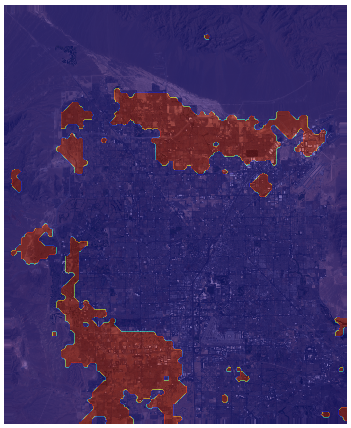 |
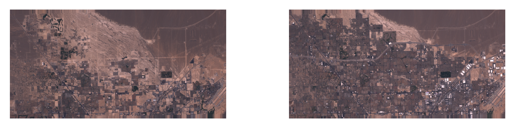
And a detailed image of North Las Vegas:
Detail Las Vegas 1999 - 2020
 |
 |
The self-supervised method demonstrated a better generalization capability on new data downloaded from another satellite mission with similar GSD. This lightweight model can easily run on AWS-EC2 instance and perform inference on big areas —for example the state of Alaska which is 1,481,346[Km2] * 0.000304907[$/km2] = $451.67. This way we define in a more economical way the areas that need to be analyzed in more detail.
Conclusions
Detecting Earth's changes from satellite imagery can be an expensive task when applied to high-resolution imagery of the entire world. As we have seen here, one way to ease this computational effort is to select some areas where the greatest changes have occurred by looking at the low-resolution image. Then look at the selected location with the high-resolution image and perform a more complex analysis, such as the segmentation of buildings or the search for roads not present in the GIS maps. We at GA-CCRi think that this kind of techniques can lead to a cheaper satellite imagery processing and imagery collection, essential to develop new optimal solutions.
We saw why supervised training is not scalable for this task: out of 24 low resolution images from the ONERA dataset, 308825 pixels have been annotated by hand from the about 10^6 total pixels in the images. This translates into many hours and a great effort made by a group of people. However, we must consider how manual work to annotate these images is error-prone to classification errors. A commercial satellite mission like Landsat can collect 532 images every day. This is about 170 km per side of each square image—since April 15, 1999 about 4 * 10 ^ 6 images of 8000x8000 pixels. We don't want to annotate such a large number of images by hand. Using a self-supervised methodology shows another approach that is more scalable to data and which generalizes better to real-world imagery. As we saw above, we can frame the change detection problem by using a weakly annotated dataset and a ranking loss function.
In the next blog post we will see how to train an unsupervised Fully Convolutional Network model using raw images downloaded directly from Landsat. All these concepts of ranking loss and triplet mining are essential for a deeper understanding. The data will be downloaded directly from the Landsat database, so they must be preprocessed. We will see how the task becomes increasingly challenging when using raw real-world data, which introduces greater variability. We will demonstrate a possible solution to clean up the data, train the model and run the inference on a new data.
References
- Deep learning in remote sensing: a review, Xiao Xiang Zhu et al. ,https://arxiv.org/abs/1710.03959
- A Survey of Change Detection Methods Based on Remote Sensing Images for Multi-Source and Multi-Objective Scenarios by Yanan You et al. , https://www.mdpi.com/2072-4292/12/15/2460
- Landsat: https://ers.cr.usgs.gov/
- SAR implementation: https://arxiv.org/abs/2104.06699
- EuroSat dataset: https://arxiv.org/abs/1709.00029
- EarthNet2021: https://arxiv.org/abs/2104.10066
- Urban Change Detection for Multispectral Earth Observation Using Convolutional Neural Networks Rodrigo Caye Daudt et al. : https://arxiv.org/abs/1810.08100%
- FaceNet: A Unified Embedding for Face Recognition and Clustering, Florian Schroff et al. : https://arxiv.org/abs/1503.03832
- Understanding the Amazon from Space, Yiqi Chen et al. , http://cs231n.stanford.edu/reports/2017/pdfs/912.pdf
- Self-Supervised Learning of Pretext-Invariant Representations, Ishan Misra et al. , https://arxiv.org/abs/1912.01991
- https://gisgeography.com/sentinel-2-bands-combinations/
- https://sentinels.copernicus.eu/web/sentinel/user-guides/sentinel-2-msi/resolutions/spatial
- Copernicus Open Access Hub: https://scihub.copernicus.eu/
- ESA(EUROPEAN SPACE AGENCY): https://sentinel.esa.int/web/sentinel/home