Bootstrapping a Better Model

Modern computer vision models often do a fantastic job of identifying the contents of an image, but they can also make mistakes, confusing one type of object with another. These mistakes sometimes make human-interpretable sense, but other times the reason for the mistake is less than obvious. In either case, however, the field has developed useful approaches for reducing this confusion and improving model performance. One approach is an iterative process called Negative Mining, where we use the model’s errors to make the model itself better.

Negative mining

When we ask a model to identify the contents of an image, it’s important that a model not only knows what an object is, but also what the object is not. It’s a subtle distinction, but without negative examples (that is, images of things we don’t want to detect), models struggle to distinguish classes of interest from other objects that we want to ignore. In a perfect world, the data you use to train your model should contain examples of the objects you care about, as well as examples of all of the other types of things the model may see.

In the real world, our training data is rarely this comprehensive. One major downside of training data that lacks representative negative examples is that the model may produce a lot of false positives when it is exposed to data not in its training set. Negative mining is the process of taking these false positives, using them to augment the original training data, and then performing additional rounds of model training. Through this procedure, we can ultimately create a training dataset that more accurately maps on to real-world use cases and allows us to create models that do a better job of distinguishing positive and negative classes.

Training a bird classifier

Imagine you’re a bird watching enthusiast, and you want to set up a system to detect specific types of birds that come to your bird feeder. Ultimately, your plan is to aim a motion-triggered camera at the feeder, and every time it takes a picture, you want a computer vision model to try to identify the presence and type of bird. How would you train a classification model for your bird recognition system on a publicly available dataset of bird images?

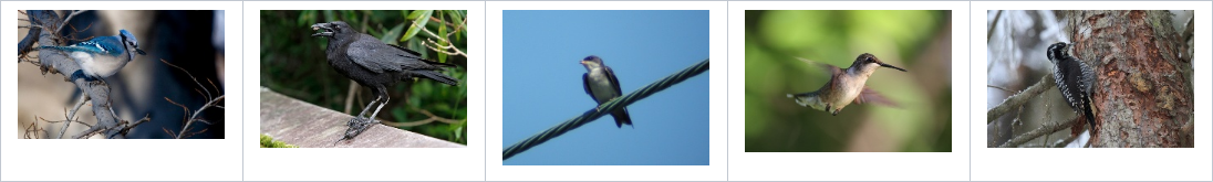
The Caltech-UCSD Birds 200 (CUB-200)1 dataset contains images of over 200 species of mainly North American birds. To simplify things, let’s assume you only want the model to detect a small subset of bird species that are of particular interest. We’ll reduce the dataset to just a handful of species, including crows, hummingbirds, swallows, blue jays, and woodpeckers. We will then group all the remaining species of birds into an “other” category. See Figure 1 for example training images.

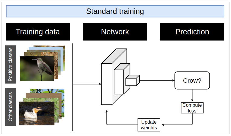
Figure 1: example training data from CUB-200. From left to right: blue jay, crow, swallow, hummingbird, woodpecker.

After holding out a small subset of the data for evaluation, we then take a pre-trained ResNet-34 model, and using PyTorch, fine-tune the model to classify an image into one of the five species or into the sixth “other” category. To train this model, we follow the the standard training paradigm of feeding the model images of different classes, evaluating the model’s output, computing the loss, and using back propagation to update the model weights. A schematic of this process in shown in Figure 2.

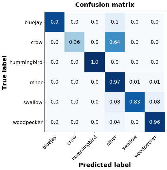
Figure 2: Standard model training procedure, illustrating a single training epoch.

After training the model for 10 epochs, the model has converged to a state where it generates reliable-looking predictions, as shown in the confusion matrix below (Figure 3). Based on the held out sample, the model performs reasonably well at categorizing the type of bird, with the exception of crows, which were often misclassified into the “other” category. Overall, the model seems to meet our goals of accurately detecting the specific birds we are interested it. However, we haven’t truly validated this model yet, as the true test of a viable model is how it behaves when exposed to real-world data.

Figure 3: Confusion matrix for the 5 categories of interest as well as the “other” category. Values indicate the proportion of test samples per class that were predicted to fall into the class indicated by the column label.

An unexpected visitor

One day you get an alert that a woodpecker is at your birdfeeder, but when you check the image of the bird, you see that it is, in fact, a squirrel. To you, this is clearly wrong. The model, on the other hand, never saw squirrels during its training and therefore doesn’t know how to classify them.

Figure 4: A squirrel at the bird feeder, misclassified as a woodpecker.

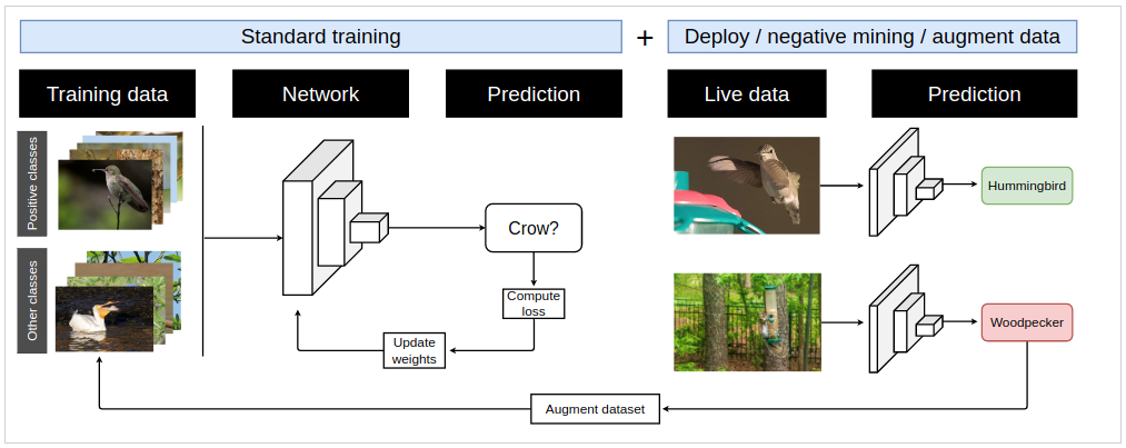
You have no interest in squirrels and only want to know when certain bird species are present. To improve the performance of the model and avoid these false positive detections, we use negative mining and the false positive images of squirrels to augment our training dataset. Specifically, we add the squirrel images to the “other” class, which represents categories of objects that are not of interest. After collecting a number of images of squirrels at the feeder that were misclassified as birds, we can retrain the model using the larger dataset. After retraining, the model no longer confuses squirrels for birds, and it correctly ignores them. A schematic of the negative mining process is shown in Figure 5.

Figure 5: Training with negative mining.

Negative mining, positive improvements

This scenario is somewhat simplistic, but it illustrates a few broad and important points about model development and deployment: your model is only as good as the data it was trained on, and it can be quite difficult to generate or find training data that is truly representative of real-world use. When applying computer vision models to live streams of data, as we do at GA-CCRi, it’s hard to know ahead of time what the model will be exposed to. Using negative mining allows us to improve model performance over time, to adapt to changing conditions, and to ensure that the models we produce are effective and beneficial to their users.

References

1. Welinder P., Branson S., Mita T., Wah C., Schroff F., Belongie S., Perona, P. “Caltech-UCSD Birds 200”. California Institute of Technology. CNS-TR-2010-001. 2010

Go Back