Algorithms for effective automated target recognition (ATR) at scale must be able to process large imagery datasets in a timely manner, while minimizing human effort in terms of annotating images and reviewing model predictions. Convolutional neural networks (CNNs) excel at many computer vision tasks, but can have a high rate of false positives under certain conditions. CNN models typically have high-dimensional input spaces, which can result in large differences in output in response to small perturbations on the input image. Consequently, anomalous and corrupted images can fool the model into producing spurious detections. Moreover, pre-training on natural imagery datasets such as ImageNet introduces rotational bias into the model.

In order to address these issues and reduce false positives, we created a novel set of CNN architectures called Synthetisc Latent Discriminative Representation (SLDR) models. As the name suggests, SLDRs are designed to replace the latent feature extraction portion of a pre-trained CNN with a smaller CNN that is generated using synthetic data. SLDR networks have several desirable properties: they use far fewer parameters than traditional CNNs and respond more smoothly to small perturbations. SLDR representations also transform uniformly under rotations of the input image, because the weights are rotationally symmetric by construction. SLDRs can detect anomalous or corrupted images by reliably separating them from normal data in the latent feature space. Furthermore, SLDRs can be ensembled with existing supervised CNNs in order to boost model accuracy and robustness to various types of noise. This blog post is based on a technical report originally published in June 2020 [3].

Latent feature extraction

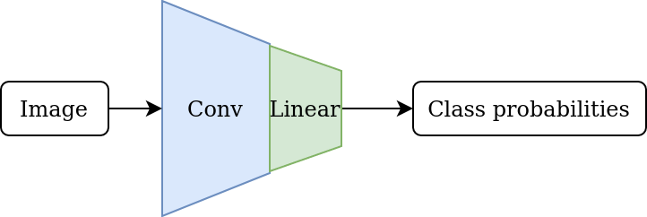
Standard transfer learning methods enable one to use existing models with lots of training and development already behind them, and repurpose those for a specific domain, via the following steps:

1.  Start with a pre-trained CNN classifier.
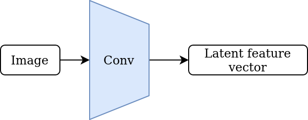
2.  Remove the final linear layer to obtain the underlying latent feature extractor.
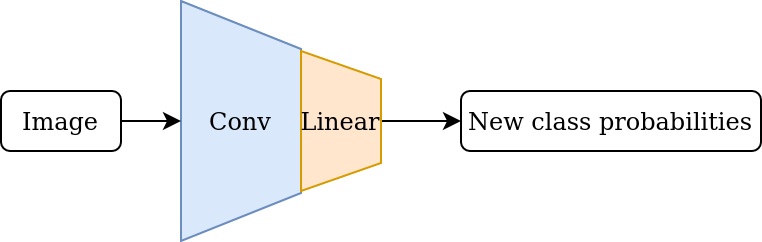
3.  Add a new linear layer aligned with the desired classes, and fine-tune the network on domain-specific training data.

The diagram below illustrates the steps of this process.

1. Pre-trained CNN	2. Latent feature extractor
3. Fine-tuned model

From this point of view, it is clear that the central object in this process is the latent feature extractor. The crucial assumption is that the feature extractor has learned to encode general-purpose image features that are useful outside of its training domain. However, typical CNN feature extractors inherit certain biases from being trained on natural imagery. For example, models that are pre-trained on ImageNet are extremely sensitive to horizontal and vertical edges due to the abundance of horizons, walls, and similar axis-aligned objects in typical natural imagery. Modern CNNs also tend to have a large number of model parameters, which increases the computational cost of training and inference.

Is it possible to design a feature extraction model which alleviates these issues, while also delivering comparable performance? This new model should have fewer parameters, be less sensitive to input perturbations, and equivariant with respect to image rotations. Our solution was to create our new SLDR models, which we will discuss in more detail below.

Effective kernels for Resnet-50 layers

In order to construct SLDR feature extractors with the desired properties, we started by deconstructing a Resnet-50 CNN [4]. Our goal was to reverse engineer the trained feature extractor, while using a minimal number of layers and adding the rotational equivariance property.

The figure below illustrates the full Resnet-50 architecture. After the initial convolution layer and associated transformations (batch normalization, Rectified Linear Unit activation, and max pooling), the model consists of four modules, each with a number of residual blocks.

Resnet-50 architecture

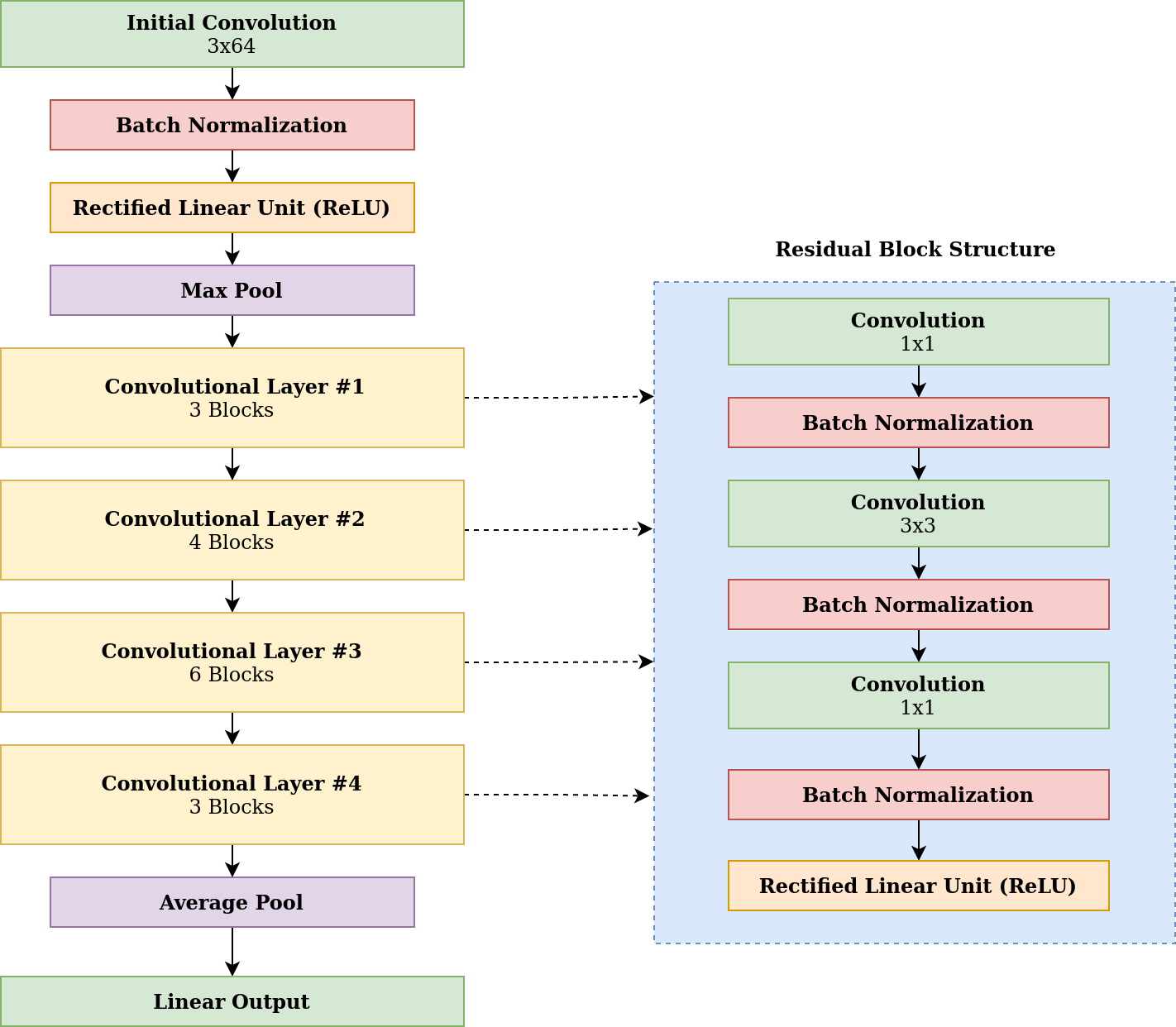Since the first convolutional layer consists of 64 7x7 kernels with three channels each, we can visualize them as 64 different RGB images. In what follows, we will think of this first layer of Resnet-50 as a one-layer latent feature extractor with 64-dimensional vector output. We will refer to this layer as "Resnet-50 Conv1".

Examples of the Resnet-50 Conv1 Kernels

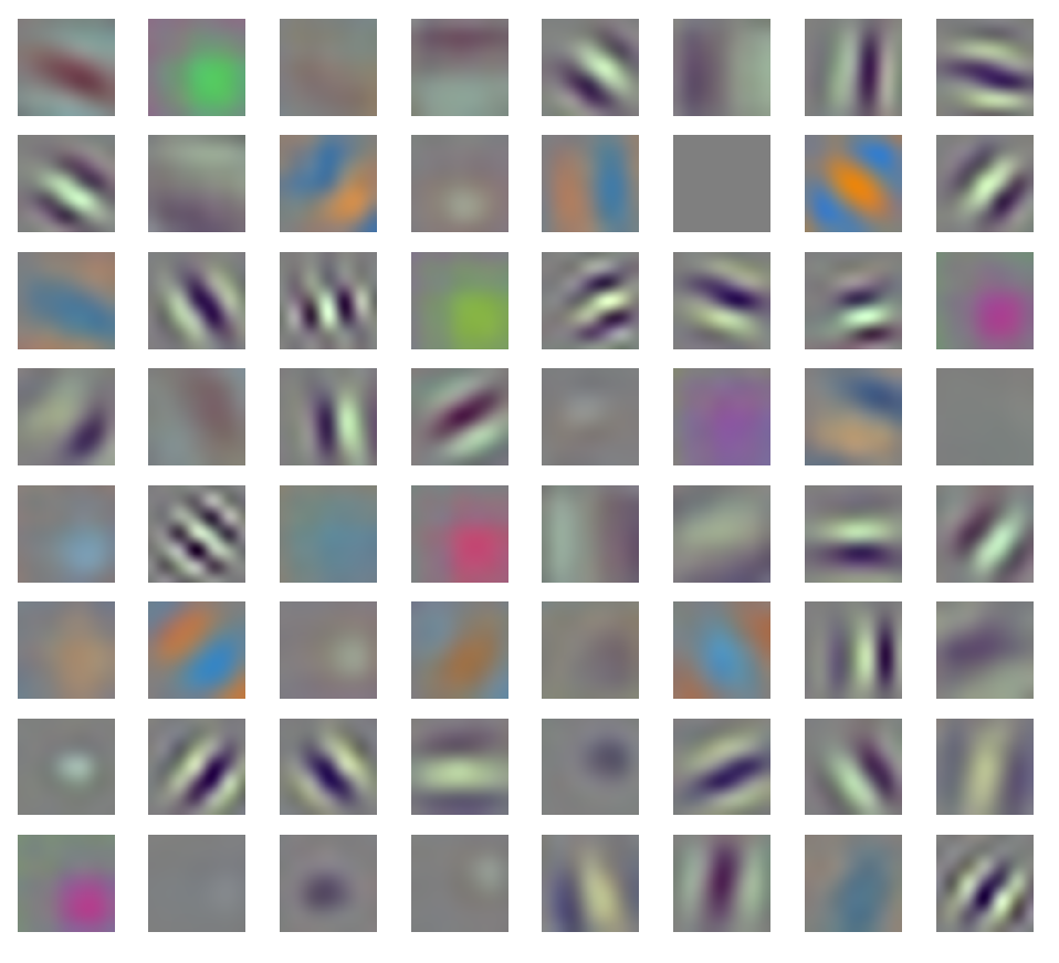Note that these 64 kernels have a dual nature: they are 7x7 pixel RGB images, and they also correspond to a latent feature extractor. We exploit this duality by passing these images through the model that they represent. The plot below shows a 3D PCA plot of the resulting vectors.

PCA of Resnet-50 conv1 kernel images passed through the first layer of Resnet-50

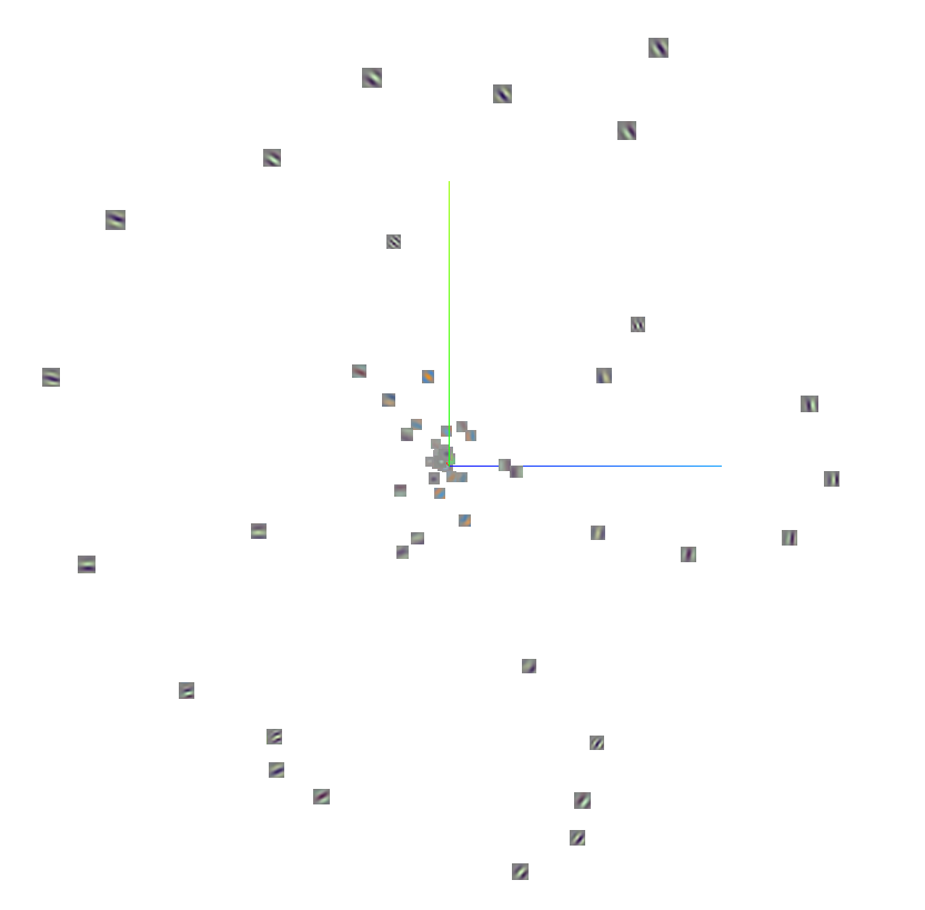There are four main clusters of data in the plot:

• Two-dimensional Gaussians (blobs)
• Orange and blue sinusoids (alternating bands of color)
• Low-frequency grayscale sinusoids (one or two wide black and white bands)
• High-frequency grayscale sinusoids (several thin alternating black and white bands)

Also note that the sinusoids do not continue to the edge of the image, but are attenuated by what appears to be a Gaussian envelope. Two-dimensional sinusoids with Gaussian envelopes are also known as Gabor wavelets. In fact, all 64 of the Resnet-50 Conv1 kernels can be derived as special cases of Gabor wavelets. The figure below illustrates how learned kernels can be approximated by synthetic Gabor wavelets.

Kernel type	Resnet-50 kernel (left) and Gabor kernel (right)
Gaussian
Low-frequency sinusoid
High-frequency sinusoid - central peak
High-frequency sinusoid - central valley

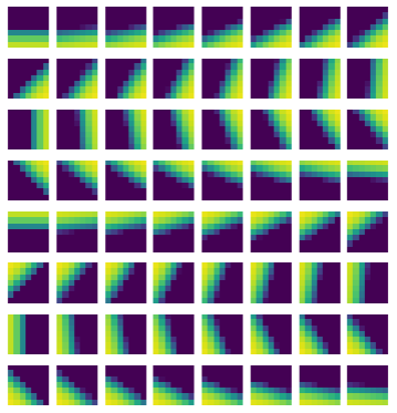
Furthermore, the effective kernels for the deeper Resnet layers are simply combinations of these 64 Gabor wavelets. Therefore, we can apply the corresponding transformations to these images to visualize the effective kernels within each sub-layer. For example, the table below shows the kernels for the first convolutional layer of Block 0 in Module 4. Note that the grayscale Gabor wavelets and their linear combinations seem to dominate in the network's output.

Resnet-50 effective kernels for Module 4, Block 0, Layer 1

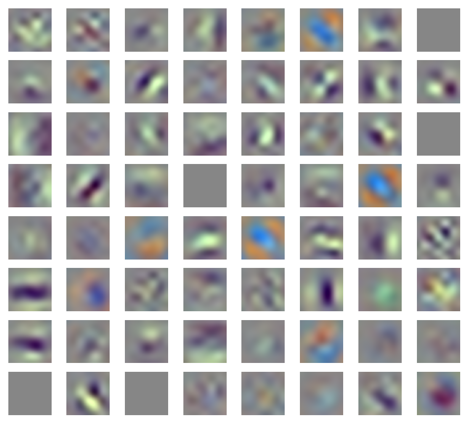Next we generate synthetic kernels from two-dimensional sinusoids, and take their linear combinations. The plots below show 16 sinusoids with varying orientation and phase, along with all of their pairwise sums. Note the similarity between these and the Resnet kernels visualized above.

16 two-dimensional sinusoids	Pairwise sums of the 16 given sinusoids

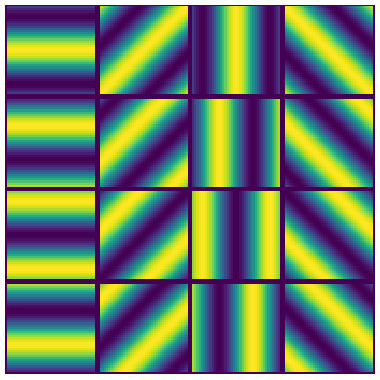The visualizations suggest that learned CNN kernels can be approximated by algebraic operations involving Gabor wavelets.

Feature extraction via sigmoids

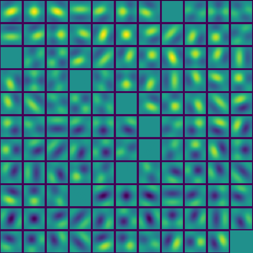
While sinusoids are similar to learned CNN kernels, there is an even simpler class of synthetic kernels, namely two-dimensional sigmoids. The figure below shows 64 sigmoid kernels with varying orientations. We refer to a one-layer CNN with sigmoid kernels as SK1.

Example of SK1 kernels

To compare SK1 and Resnet-50 Conv1 as feature extractors, we generated classes of synthetic images, and then passed them to each output. We then used PCA to visualize the structure of these embeddings to see how the models fared at distinguishing patterns. The results for some of these tests are below.

Corners with varying angles

PCA of SK1 feature vectors	PCA of Resnet-50 Conv1 feature vectors

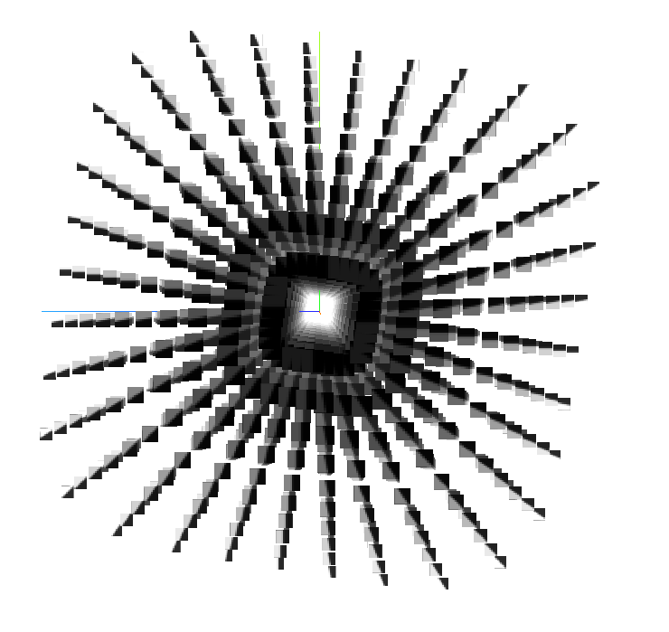
The space of angles forms a rhombic dodecahedron, which is clearly visible in the SK1 feature vectors. Resnet-50 Conv1 then flattens this polyhedron into a disk shape.

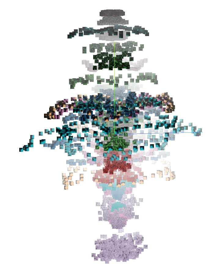
Edges with varying dynamic range

PCA of SK1 feature vectors	PCA of Resnet-50 Conv1 feature vectors

The space of edges with varying dynamic range forms a solid octahedron, which is faithfully represented by SK1. Resnet-50 Conv1 again flattens the polyhedron.

Line segments

PCA of SK1 feature vectors	PCA of Resnet-50 Conv1 feature vectors

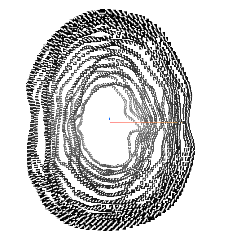The space of line segments forms a Mobius band, which is again well-represented by SK1. Resnet-50 Conv1 collapses the space and does not preserve the topological structure.

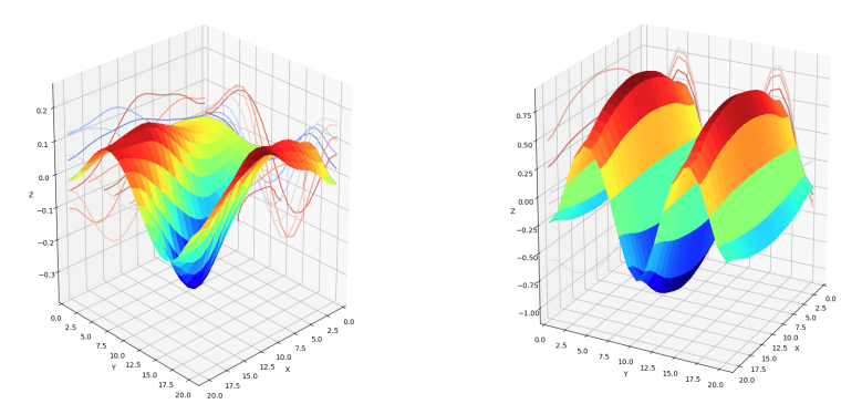
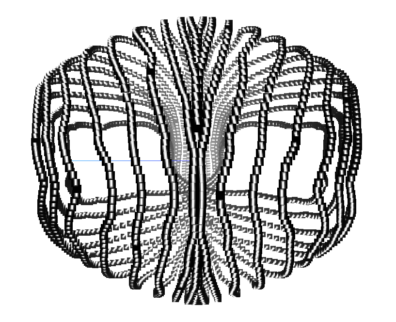
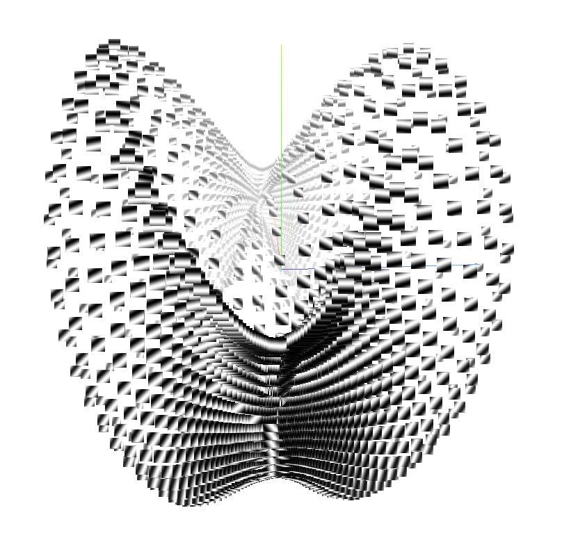
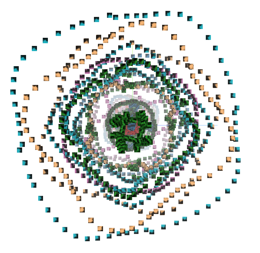
Two-dimensional Sinusoids with a Fixed Frequency

PCA of SK1 feature vectors	PCA of Resnet-50 Conv1 feature vectors

For a fixed frequency, the space of two-dimensional sinusoids forms a Klein bottle [1], the outlines of which are discernible in the SK1 representation. On the other hand, Resnet-50 Conv1 does not seem to properly represent the topological features.

Consistently, the SK1 model was able to preserve the structure of the input features better than Resnet-50 Conv1. These visualizations provide qualitative evidence that representations using synthetic kernels may be useful for complementing learned representations.

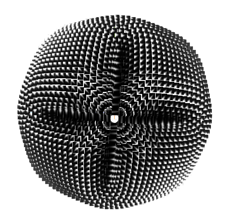
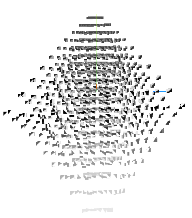
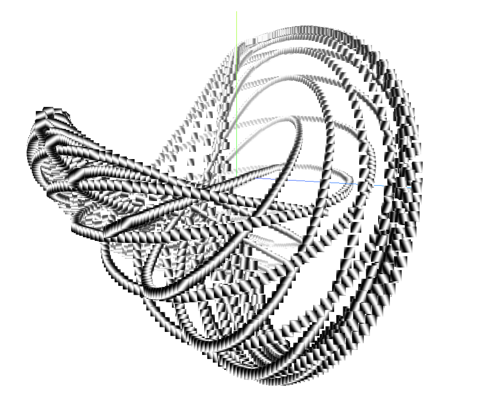
The SK1 model also produces representations that are rotationally equivariant, since the kernels are chosen to uniformly cover all possible orientations. When a model is rotationally equivariant, rotating an image transforms the feature vector along a corresponding rotation in higher dimensions. To give evidence for this property, we rotated and vectorized center crops of several images from the UC-Merced Land Use dataset [7]. The corresponding PCA plots are shown below. The rotational equivariance of SK1 is visibly apparent in the plot, while we note that Resnet-50 Conv1 collapses the representations of the rotated images.

PCA of SK1 feature vectors	PCA of Resnet-50 Conv1 feature vectors

The above plots suggest that SK1 represents certain local features of images more faithfully than the first layer of Resnet-50. Next we consider more general SLDR models.

Performance of Gabor wavelet SLDRs

The construction of a one-layer SLDR model involves sampling a set of kernels from the space of Gabor functions, which is parameterized by orientation, phase, and frequency. For the deeper layers, we generate synthetic convolutional layers that consist of orthogonal combinations of the kernels from the first layer.

Ensembled models

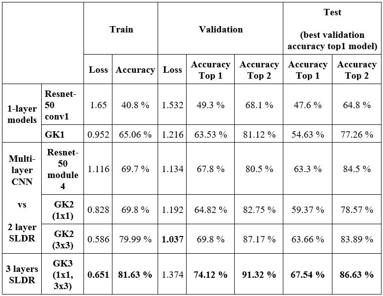
In order to evaluate the accuracy of SLDR models relative to Resnet-50, we trained linear layers on the feature vectors of each model for three land use classification tasks. First, we tested the synthetically generated models as standalone classifiers by comparing the top-1 accuracy of a SLDR model with two convolutional layers relative to module four of Resnet-50, which has ten convolutional layers. Next, we ensembled Resnet-50 with a SLDR model and measured the accuracy relative to Resnet-50 on two datasets: the UC-Merced Land Use Dataset and the Describable Textures Dataset [2]. For the last test, we compared the robustness of Resnet-50 and the ensembled SLDR model. The images for this test were 64x64 pixel crops from seven classes selected from the UC-Merced Land Use dataset. To avoid introducing bias due to correlation between land use classes and colors, we only used grayscale images for testing.

Accuracy of standalone models

First, we measured the performances of the standalone synthetic networks on 64x64 pixel crops from the UC-Merced dataset. We find that models with just two synthetically generated layers rival the performance of module 4 of Resnet-50. In the table below, the SLDR models derived from Gabor kernels are denoted with the prefix GK, followed by the number of layers. The first layer in each model has 96 kernels. The following layers are either 1x1 conv or 3x3 conv layers. Each conv layer is followed by a ReLU layer. Note that our SK1 and GK1 models are similar to the circle and Klein layers introduced in [6].

Accuracy of ensembled models

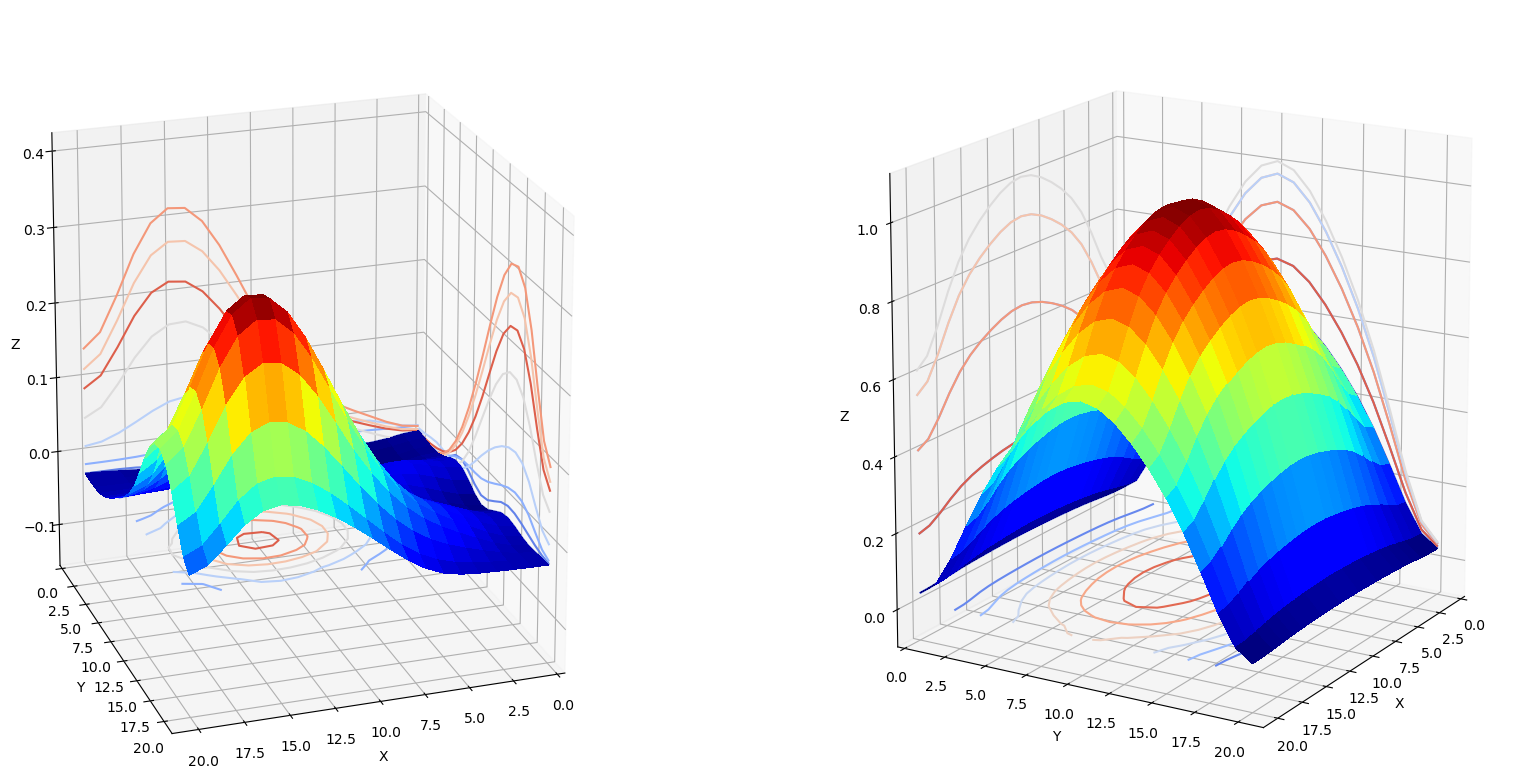
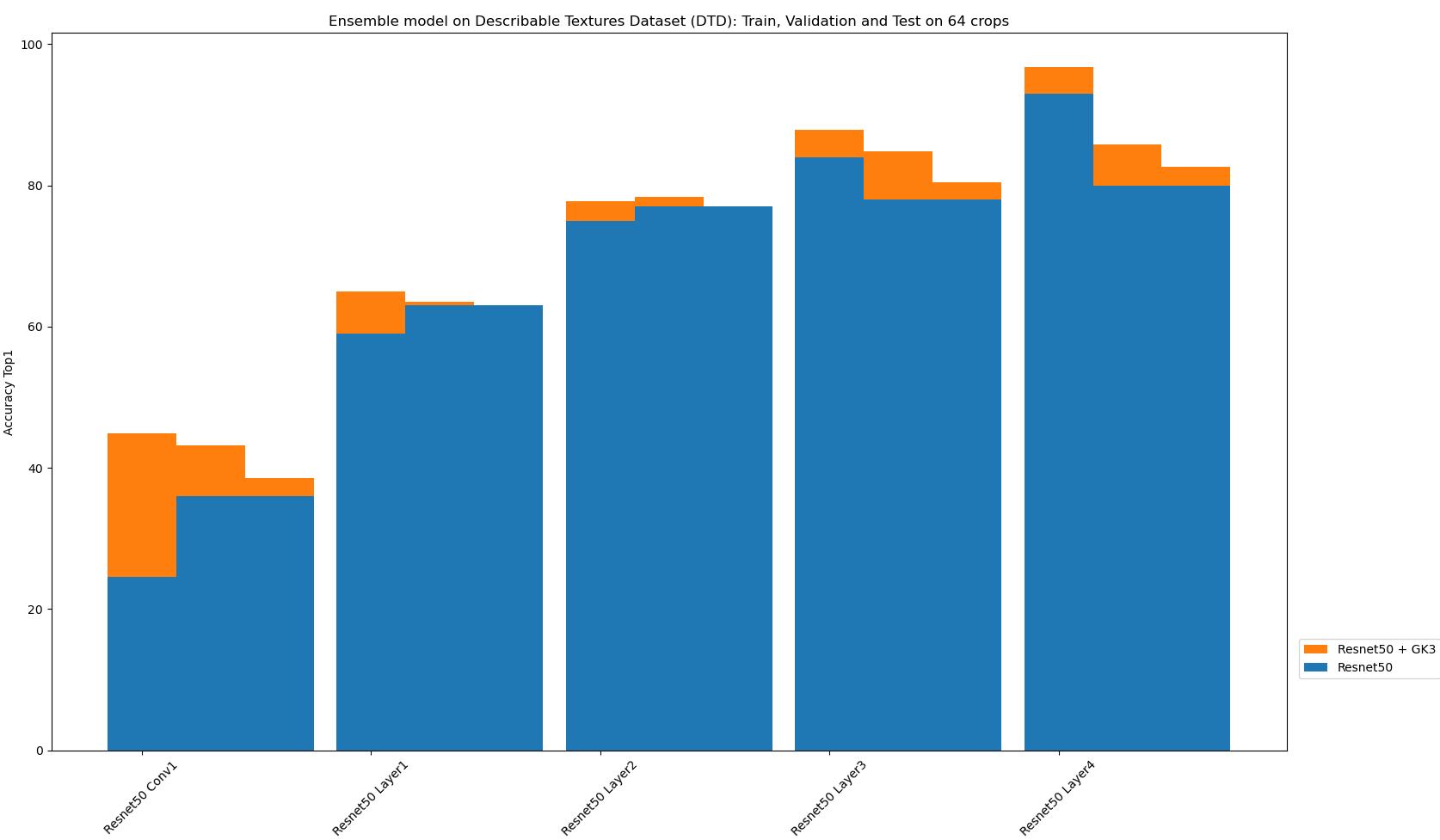
We ensembled feature extraction models by training a linear layer on the concatenation of their feature vectors. To build the first evaluation dataset, we combined a subset of the UC-Merced classes into super-classes that are highly visually distinguishable: agricultural, airplane, buildings, scrubland, natural (such as forests and rivers), parking lot, and roads. We took several 64x64 pixel crops from each super-class. The figure below shows the top-1 accuracy (over training, validation, and test sets) for Resnet-50 sub-layers (blue) as well as their respective GK3 ensembles (orange). Note that the PyTorch library refers to Resnet-50 modules 4-7 as "layers" 1-4, which is the notation used in the plot below. We find that at each level, ensembling with the GK3 model improves overall classifier performance.

Training, Validation and Test Accuracy on UC-Merced crops for 7 classes

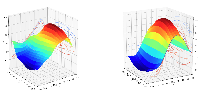
In the interest of testing the generalization of SLDR models, we repeated the above experiments using the Describable Textures Dataset. As shown in the figure below, we found that ensembling with GK3 boosts accuracy for each sub-layer of Resnet-50.

Training, Validation and Test performances on DTD crops 64 for 5 classes

Model robustness to corruption

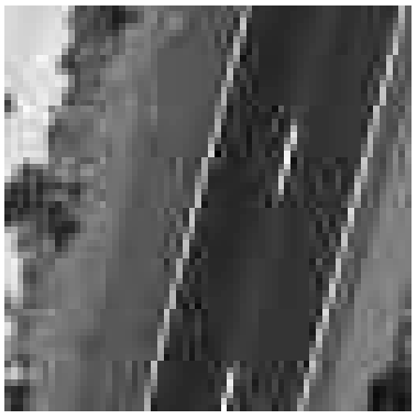
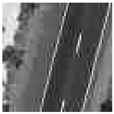
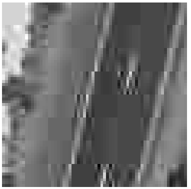
In order to further test the robustness of our results, we evaluated model accuracy relative to five different types of image corruptions [5]:

• Additive White Gaussian Noise (AWGN)
• Pixelation
• JPEG
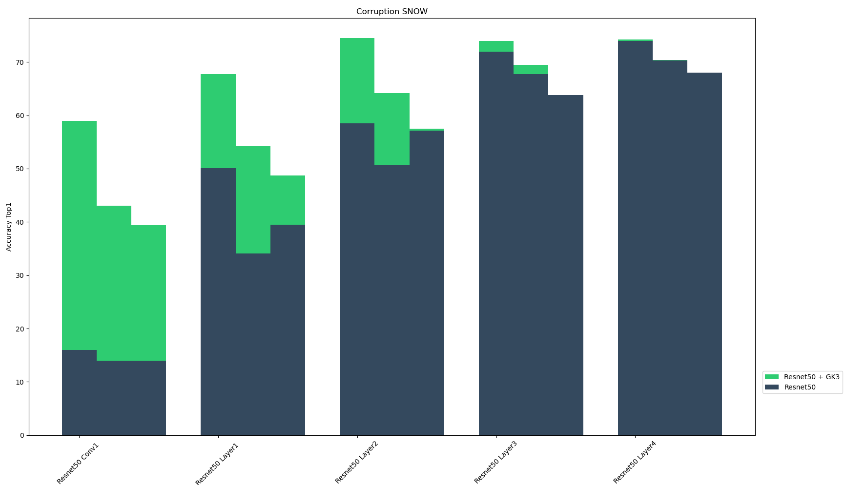
• Snow
• Frosted glass blur

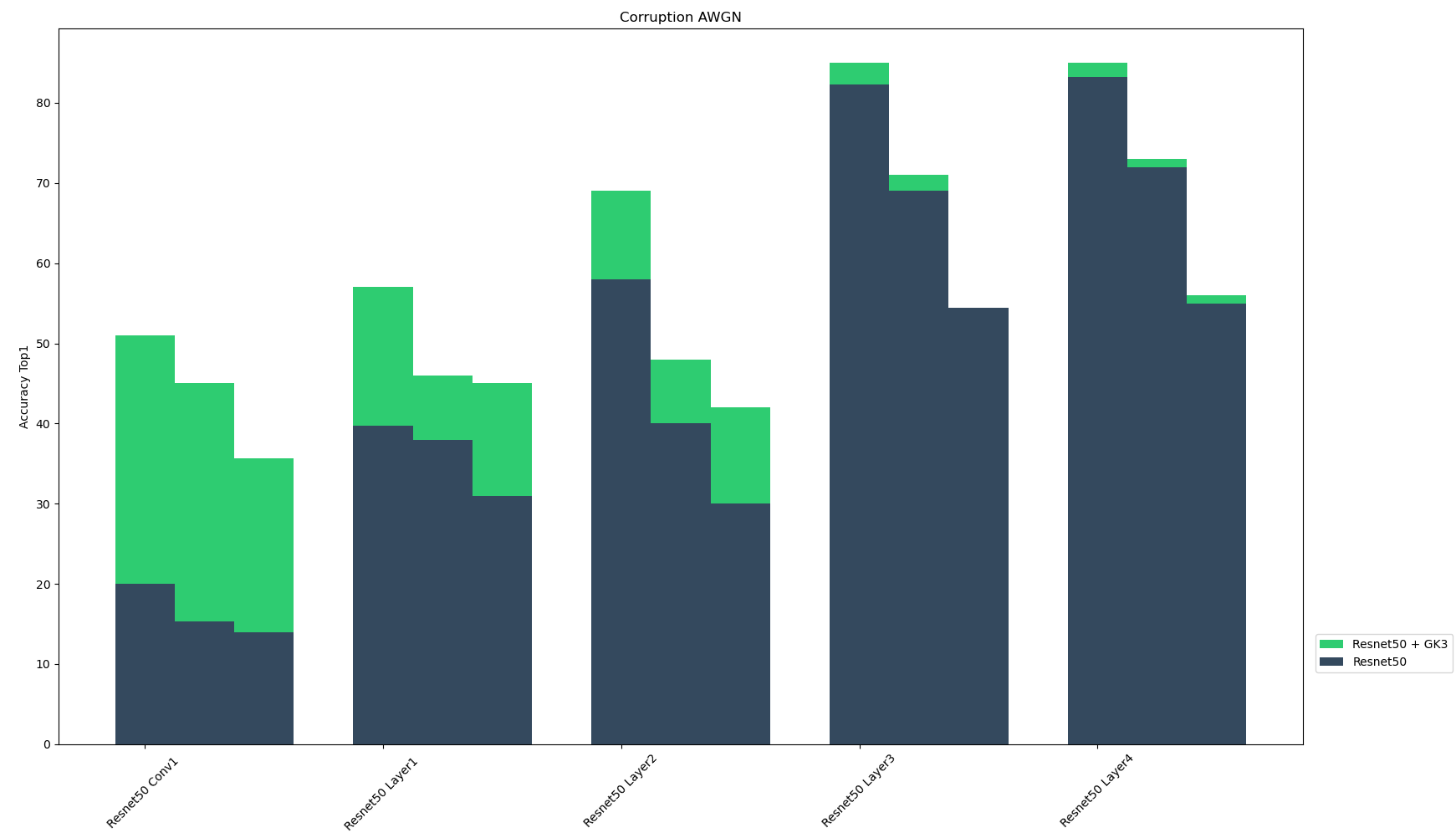
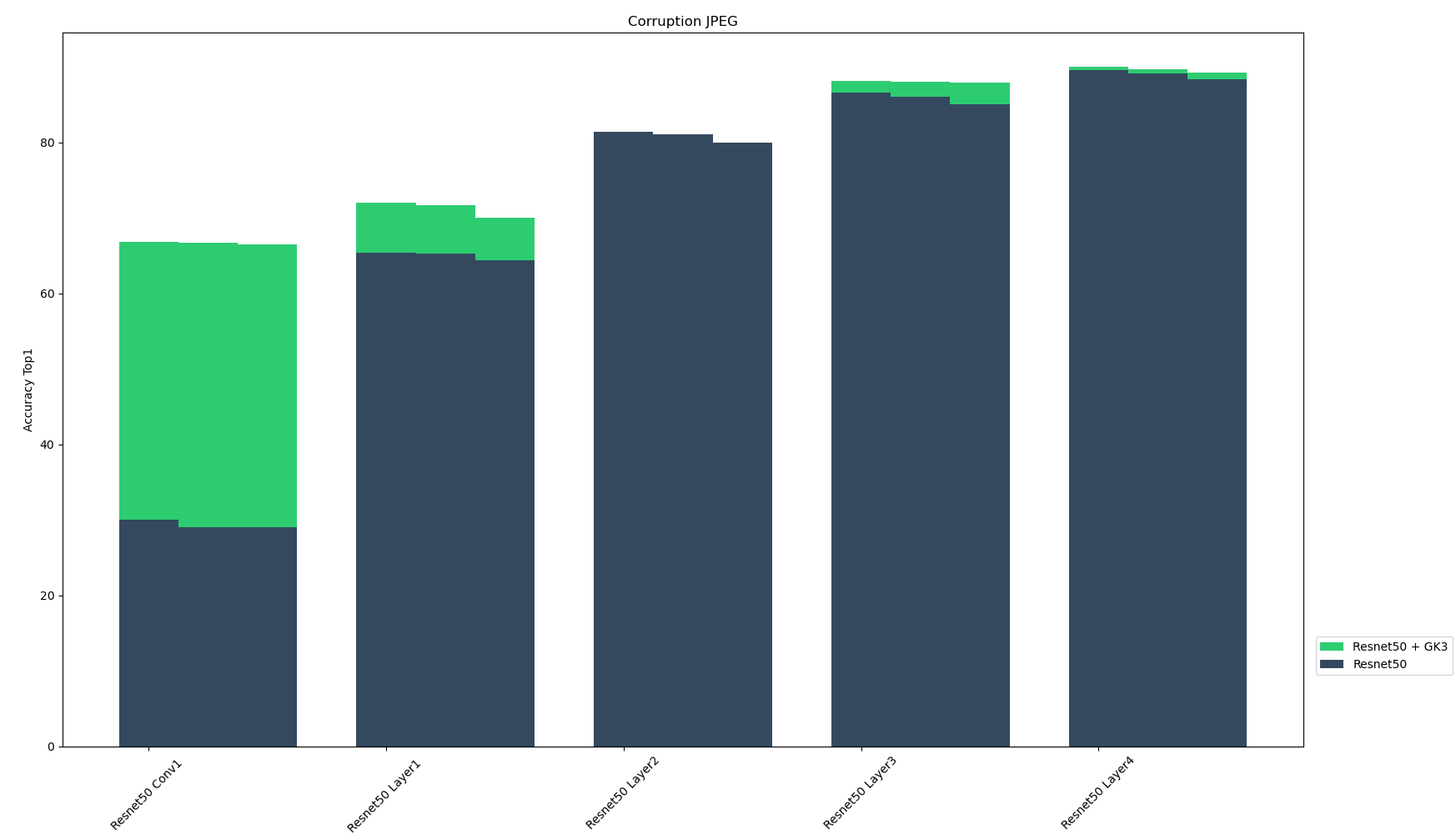
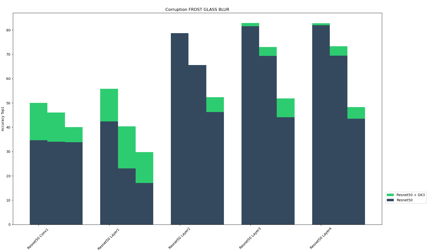
These algorithmically generated corruptions derive from three different categories: added noise, digital loss, and natural weather perturbation. Each type of corruption has three levels of severity, resulting in fifteen distinct corruptions. For each of the five corruption techniques, the figure below shows the the top-1 accuracy of Resnet-50 sub-layers and their GK3 ensembles for the three corruption severity levels. We found that the ensemble models enhance model performance across multiple layers and corruption types. Ensembling with SLDR models seems to make the models more resilient to corrupted inputs.

AWGN	Top-1 accuracy of Resnet-50 sub-layer and GK3 ensembles over three corruption severity levels
Pixelate	Accuracy Top 1
JPEG	Accuracy Top 1
Snow	Accuracy Top 1
Frosted glass blur	Accuracy Top 1

Final Thoughts

SLDRs increase model accuracy, while also improving their resilience to image corruption and perturbations. Additionally, SLDRs are rotationally equivariant, which makes their outputs less biased to image rotations. When building upon pre-trained models, one must think carefully about bias introduced by training data, as well as the properties of the target domain. By digging deeper into model architectures, we were able to create compact, robust CNNs with discriminative power comparable to larger networks.

References

1. Carlsson, G. et al. (2008). On the Local Behavior of Spaces of Natural Images. International Journal of Computer Vision 76, 1-12.
2. Cimpoi M. et al. (2014). Describing Textures in the Wild. Proceedings of the IEEE Conf. on Computer Vision and Pattern Recognition (CVPR).
3. Dhand V., and Graziani A., (2020). Anomaly Detection and Ensemble Robustness via Synthetic Latent Discriminative Representation (SLDR) Networks. Technical Report.
4. He, K. et al. (2015). Deep Residual Learning for Image Recognition. https://arxiv.org/abs/1512.03385
5. Hendrycks, D. and Dietterich, T. (2019) Benchmarking Neural Network Robustness to Common Corruptions and Perturbations. International Conference on Learning Representations (ICLR).
6. Love, E. et al. (2021). Topological Deep Learning. https://arxiv.org/abs/2101.05778
7. Yang, Y. and Newsam S. (2010). Bag-Of-Visual-Words and Spatial Extensions for Land-Use Classification. ACM SIGSPATIAL International Conference on Advances in Geographic Information Systems (ACM GIS).