GA-CCRi Analytical Development Services

There are many reasons that researchers analyze maritime traffic. For example, commodity traders analyze the flow of goods, port operators coordinate ground transportation and minimize vessel time in port, and government agencies track economic statistics. Regardless of the use case, accurately predicting and reporting when vessels enter and exit ports is paramount.

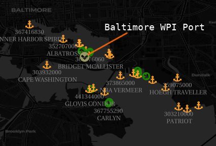
The basis of this analysis is the World Port Index (WPI), which our Optix platform includes as a geographic port layer. We found one element of this data set lacking: ports are represented by a single point, which provides no information about the port’s effective geographic extent. This is especially relevant for determining what vessels are in port, which is useful data for tracking where those vessels have traveled as well as for building analytics related to the port itself.

To improve upon the WPI’s lack of spatial resolution, we set out to apply a data-driven approach to port boundaries, applying several clustering techniques to a large corpus of historical maritime data that we had in our Optix platform.

The Data

The positional data used for this initiative was from the Automatic Identification System (AIS), a global positional system used by vessels. Vessels use AIS when emitting their location and other navigational metadata to other vessels. We have real-time and historical AIS data from our partner exactEarth, which leverages satellites and terrestrial collectors to gather that data and create a global picture of all vessels.

To trim down the data to a more manageable size, we filtered it down to only vessels with indicators that they were in port. This resulted in a data set of 812,593,583 observations.

As the base for our investigation we used World Port Index data. This data is primarily used for navigation, and provides both the location of ports as well as an abundance of metadata.

Clustering

With the AIS data collected, we set off to create port boundaries from the data locations. We tried a couple of different clustering methods before settling on Density-based spatial clustering of applications with noise(DBSCAN). DBSCAN performs clustering in an unsupervised manner by aggregating points together into core points, which must be within a set distance of a set number of other points. Any point within that set distance of those core points is considered within the cluster. If a point isn’t within any core points, then it is marked as an outlier.

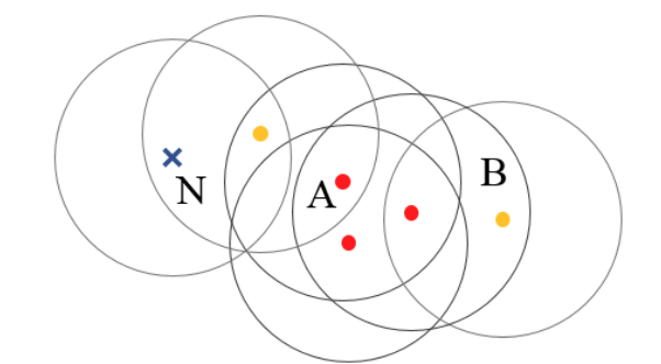
This clustering method has a number of advantages. The density-based approach means that DBSCAN can capture clusters of any shape, and its tendency to ignore outliers is also useful. DBSCAN can also be easily implemented with haversine distance, which provides a more accurate spatial measure of the data (due to these points being located on a sphere). We ran DBSCAN over the filtered data, and after tuning hyper-parameters to optimally fit the WPI, we created clusters from the data we collected.

Once we had our clusters, we constructed port polygons by calculating the convex hull for each cluster and then buffering it slightly. Once done, we could associate the polygons with the WPI port points and label the polygons. If multiple ports were within a polygon, we split up that polygon into individual ports. If there was no cluster close enough, we created a circular buffer around the WPI point as a generic boundary.

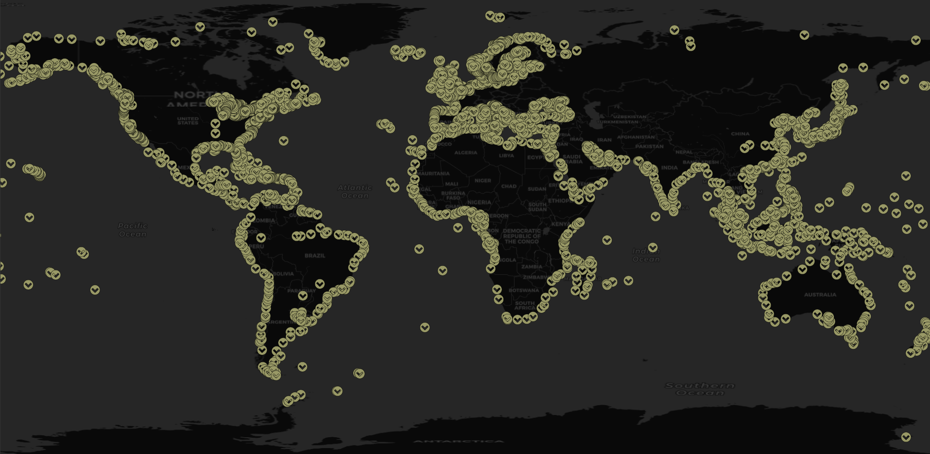
Here’s what the results look like, shown with vessels that reported as moored:

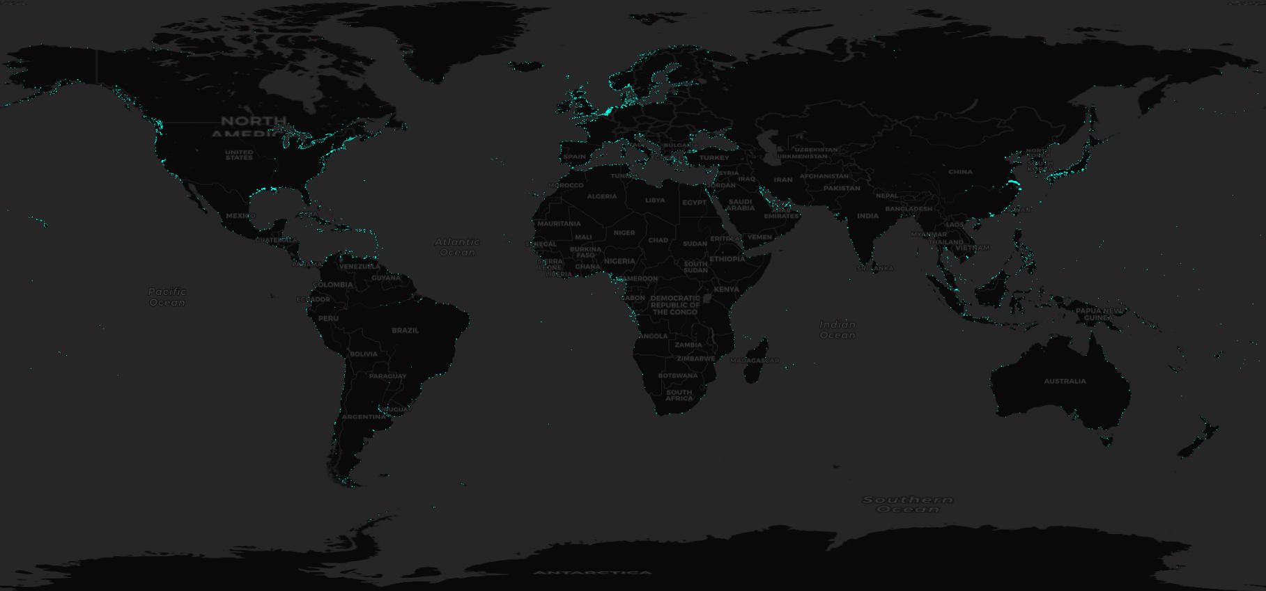
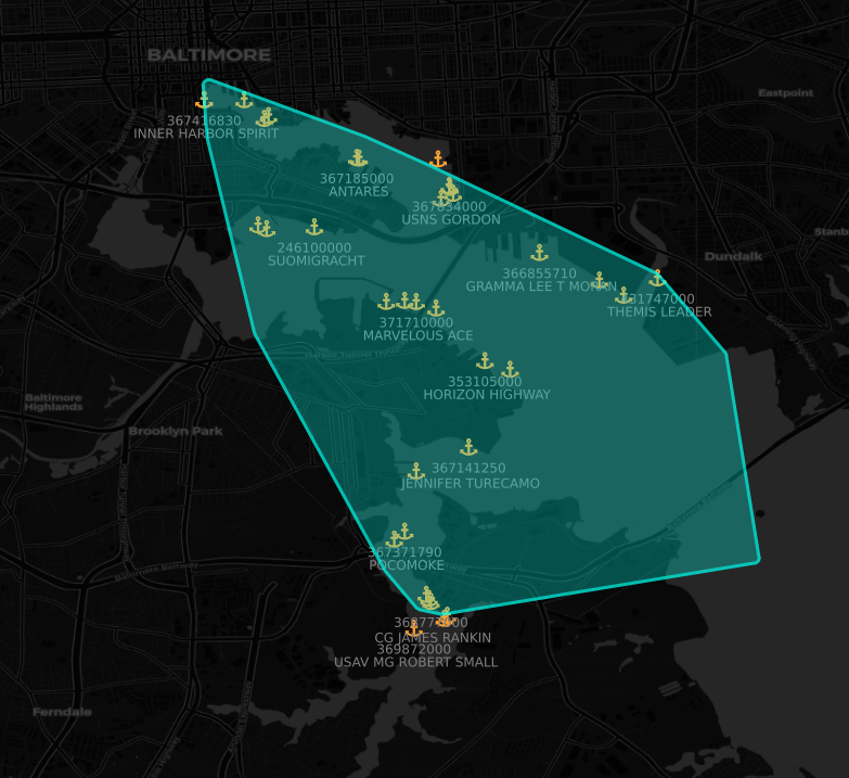
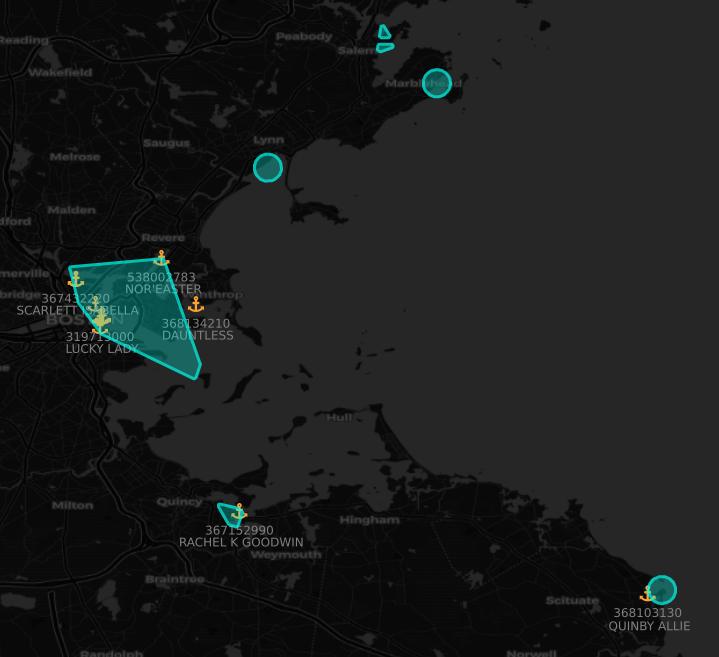
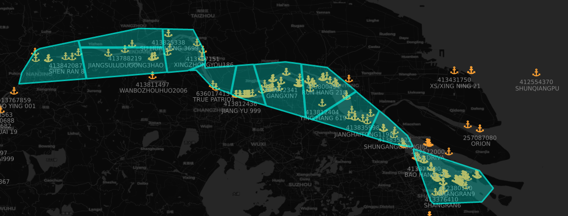
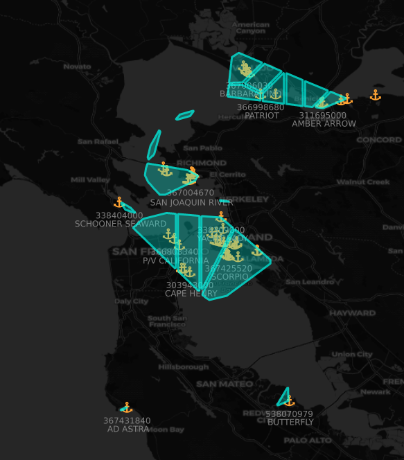
Starting with just a dataset of vessel locations, we were able to construct an accurate and comprehensive worldwide picture of all active ports contained within the WPI. This enriched layer will provide a good basis for port analytics going forward and help expand our maritime capabilities, allowing for more in-depth analytics and insights. We are excited to see what we’ll be able to build going forward with this data as it fuels other initiatives such as ETA prediction for vessels, route analysis, and port capacity evaluation.